Behavior Analytics

What motivates individuals to join an online group? When individuals abandon social media sites, where do they migrate to? Can we predict box-office revenues for movies from tweets posted by individuals? These questions are a few of many examples in which we are interested in analyzing or predicting behaviors on social media.

Individuals exhibit different behaviors in social media. These behaviors can be individual behavior or part of a broader collective behavior. When discussing individual behavior, our focus is on one individual. Collective behavior emerges when a population of individuals behave in a similar way, with or without coordination or plan.

When discussing individual and collective behavior, we provide examples of these behaviors, and elaborate techniques of analyzing, modeling, and predicting these behaviors.

10.1 Individual Behavior

We read online news, comment on posts, blogs, and videos, write reviews for products, post, like, share, tweet, rate, recommend, listen to music, and watch videos, among many other daily behaviors that we exhibit on social media. What are the types of individual behavior that result in leaving a trace on social media?

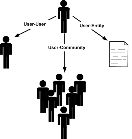
By analyzing these online behaviors, we can generally categorize individual behavior into 3 categories (shown in Figure 10.1):

• User-User Behavior. This is the behavior individuals exhibit with respect to other individuals. For instance, when befriending someone, sending a message to another individual, playing games, following, inviting, blocking, subscribing, or chatting, we are demonstrating a user-user behavior.

• User-Community Behavior. The target of this type of behavior is a community. For example, joining or leaving a community, becoming a fan of a community, or participating in its discussions are considered user-community behavior.

• User-Entity Behavior. The target of this behavior is an entity in social media. For instance, it includes writing a blogpost or review or uploading a photo to a social media site.

As we know, link data and content data are frequently available on social media. Link data represents the interactions users have with other users and content data is generated by users when using social media. One can think of user-user behavior as users linking to other users and user-entity behavior as users generating and consuming content. Users interacting with communities is a blend of linking and content generation behavior, where one can simply join a community (linking), read or write contents for a community (content consumption and generation), or can demonstrate a mix of both activities. Link analysis and link prediction are commonly used to analyze links and text analysis is designed to analyze content. We employ these techniques to analyze, model, and predict individual behavior.

10.1.1 Individual Behavior Analysis

Individual behavior analysis aims to understand how different factors affect individual behaviors observed online. In other words, behavior analysis aims at correlating these behaviors (or their intensity) with other measurable characteristics of users, sites, or contents that could have possibly resulted in the behavior.

We discuss an example of behavior analysis on social media and demonstrate how this behavior can be analyzed. After which, we outline the process that can be followed to analyze any behavior on social media.

Community Membership in Social Media

Users often join different communities in social media. The behavior of community membership is an example of user-community behavior. Why do users join communities? In other words, what factors affect the community joining behavior of individuals?

To analyze community joining behavior, we can observe users who join communities and determine the factors that are common among these users. Hence, we require a population of users U=\{u_1,u_2,\dots,u_n\}, a community C, and community membership information, i.e., users u_i \in U that are members of C. The community need not be explicitly defined. For instance, one can think of individuals buying a product as a community and people buying the product for the first time as individuals joining the community. To determine users who have already joined the community, we need community memberships at two different times: t_1 and t_2, t_2 > t_1. At t_2, we determine users such as u that are currently members of the community, but were not members at t_1. These joined users form the sub-population that is analyzed for community joining behavior.

To determine factors that affect community joining behavior, we can design hypotheses based on different factors that describe when community joining behavior takes place. We can verify these hypotheses by using data available on social media. The factors utilized in the validated hypotheses describe the behavior under study best.

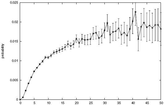
One such hypothesis is that individuals are inclined towards an activity when their friends are engaged in the same activity. Thus, if the hypothesis is valid, a factor that plays a role in users joining a community is their number of friends that are already members of the community. In data mining terms, this translates to utilizing the number of friends of an individual in a community as a feature to predict whether the individual joins the community (i.e., class attribute). Figure 10.2 depicts the probability of joining a community with respect to the number of friends an individual has that are already members of the community. The probability increases as more friends are in a community, but a diminishing returns

Diminishing
Returnsproperty is also observed, meaning that when enough friends are inside the community, more friends have no or marginal effects on the likelihood of an individual joining the community.

Thus far we define only one feature. However, one can go beyond a single feature. Figure 10.3 lists the comprehensive features that can be utilized for analyzing the community joining behavior.

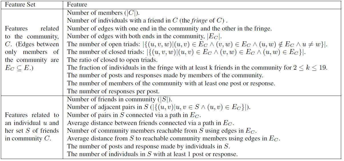
As discussed, these features may or may not affect the joining behavior; thus, a validation procedure is required to understand their effect on the joining behavior. Which one of these features is more relevant to the joining behavior? In other words, which feature can help best determine whether individuals will join or not?

To answer this question, we can utilize any feature selection algorithm. Feature selection algorithms determine features that contribute the most to the prediction of class attribute. Alternatively, we can utilize a classification algorithm, such as decision tree learning, to identify the relationship between features and class attribute (i.e., joined={Yes, No}). The earlier a feature is selected in the learned tree (i.e., is closer to the root of the tree), the more important to the prediction of class attribute value.

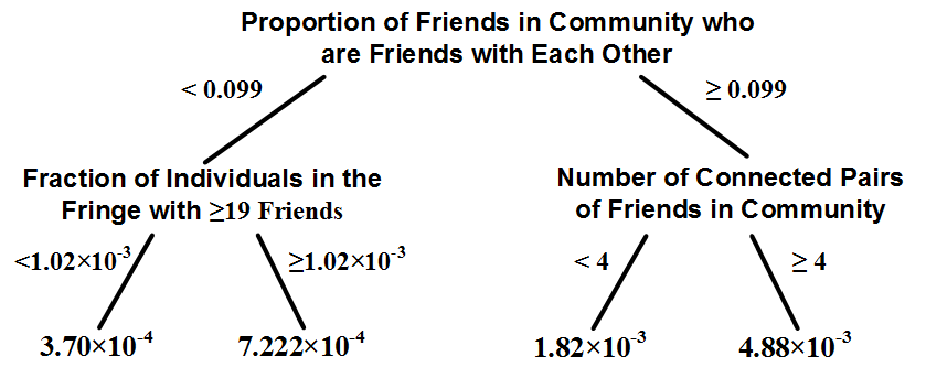
By performing decision tree learning for a large dataset of users and the features listed in Figure 10.3, one finds that not only number of friends inside a community, but also how these friends are connected to each other affects the joining probability. In particular, the denser the subgraph of friends inside a community, the higher the likelihood of a user joining the community. Let S denote the set of friends inside community C and let E_S denote the set of edges between these |S| friends. The maximum number of edges between these S friends is {|S| \choose 2}. So, the edge density is \phi(S)=E_s/{|S| \choose 2}. One finds that the higher this density, the more likely that one is going to join a community. Figure 10.4 shows the first two levels of the decision tree learned for this task using features described in figure 10.3. Higher level features are more discriminative in decision tree learning, and in our case, the most important feature is the density of edges for the friends subgraph inside the community.

To analyze community joining behavior, one can design features that are likely to be related to community joining behavior. Decision tree learning can help identify which features are better that others. However, how can we evaluate if these features are designed well and whether other features are not required to accurately predict joining behavior? Since classification is used to learn the relation between features and behaviors one can always use classification evaluation metrics such as accuracy to evaluate the performance of the learned model. An accurate model translates to an accurate learning of feature-behavior association.

A Behavior Analysis Methodology

We analyze community joining behavior. The analysis for this behavior can be summarized via a four-step methodology for behavioral analysis. The same approach can be followed for analyzing other behaviors in social media as a general guideline.

Commonly, to perform behavioral analysis, one needs the following four components:

1. An observable behavior. The behavior that is analyzed needs to be observable. For instance, consider analyzing community joining behavior. Then, the joining of individuals (and possibly their joining times) should be accurately observable to analyze it.

2. Features. One needs to construct relevant data features (co-variates) that may or may not affect (or be affected by) the behavior. Anthropologists and sociologists can help design these features. The intrinsic relation between these features and the behavior should be clear from the domain expert’s point of view. In community joining behavior, we utilized the number of friends inside the community as one feature.

3. Feature-Behavior Association. This step aims at finding the relationship between features and behavior. This relation describes how changes in features results in the behavior (or changes its intensity). We used decision tree learning to find features that are most correlated with the community joining behavior.

4. Evaluation Strategy. The final step evaluates the findings. This evaluation guarantees that the findings are due to the features defined and no externalities. We use classification accuracy to verify the quality of features in community joining behavior. To guarantee that findings are due to features and no externalities, various techniques can be utilized, such as randomization tests discussed in chapter 8. In randomization tests, we measure a phenomena in a dataset and then randomly generate subsamples from the dataset in which the phenomena is guaranteed to be removed.

   Causality
   TestingWe assume the phenomena has happened when the measurements on the subsamples are different from the ones on the original dataset. Another approach is to utilize causality testing methods. Causality testing methods measure how a feature can effect a phenomena. A well known causality detection technique is called granger causality

   Granger
   Causalitydue to Clive W. J. Granger the Nobel laureate in economics.
   

   Definition 10.1

   Granger Causality. Assume we are given two temporal variables X=\{X_1,X_2,\dots,X_t,X_{t+1}, \dots\} and Y=\{Y_1,Y_2,\dots,Y_t,Y_{t+1},\dots\}. Variable X “Granger causes" variable Y when historical values of X can help better predict Y than just using the historical values of Y.

   Consider a linear regression model outlined in Chapter 5. We can predict Y_{t+1} by using either Y_1,\dots,Y_t or a combination of X_1,\dots,X_t and Y_1,\dots,Y_t.

   Y_{t+1} = \sum_{i=1}^t a_i Y_i + \epsilon_1,(10.1)
   Y_{t+1} = \sum_{i=1}^t a_i Y_i + \sum_{i=1}^t b_i X_i + \epsilon_2,(10.2)

   where \epsilon_1 and \epsilon_2 are the regression model errors. Now, if \epsilon_2 < \epsilon_1 , it indicates that using X helps reduce the error. In this case, X Granger causes Y.

10.1.2 Individual Behavior Modeling

Similar to network models, models of individual behavior can help concretely describe why specific individual behaviors are observed on social media. In addition, they allow for controlled experiments and simulations that can help study individuals on social media.

Like other modeling approaches (see Chapter 4), in behavior modeling, one must make a set of assumptions. Behavior modeling can be performed via a variety of techniques, including techniques from economics, game theory, or network science. We discuss some of these techniques in other chapters. We review them briefly here. Interested readers are referred to respective chapters for more details.

• Threshold models (Chapter 8). When a behavior diffuses in a network, such as the behavior of individuals buying a product and referring it to others, one can use threshold models. In threshold models, the parameters that need to be learned are the node activation threshold \theta_i and the influence probabilities w_{ij}. Consider the following methodology for learning these values. Consider a merchandise store where the store knows the connections between individuals and their transaction history (e.g., the items that they have bought). Then, w_{ij} can be defined as

  w_{ij} = {\text{fraction of times user }i\text{ buys a product and}}(10.3)
  {\text{user }j\text{ buys the same product \textbf{soon} after that}}(10.4)

  The definition of “soon" requires clarification, and can be set based on a site’s preference and the average time between friends buying the same product. Similarly, \theta_i can be estimated by taking into account the average number of friends that need to buy a product before user i decides to buy it. Of course, this is only true when the products bought by user i are also bought by her friends. When this is not the case, methods from collaborative filtering (see Chapter 9) can be used to find out the average number of similar items that are bought by user i’s friends before user i decides to buy a product.

• Cascade Models (Chapter 7). Cascade models are examples of scenarios where an innovation, product, or information cascades through a network. The discussion with respect to cascade models is similar, with the exception that cascade models are sender-centric. That is, the sender decides on activating the receiver, whereas threshold models are receiver-centric, in which receivers get activated by multiple senders. Therefore, the computation of these values need to be done from the sender’s point of view in cascade models. Note that both threshold and cascade models are examples of individual behavior modeling.

10.1.3 Individual Behavior Prediction

As discussed previously, most behaviors result in newly formed links in social media. It can be a link to a user, as in befriending behavior, a link to an entity, as in buying behavior, or a link to a community, as in joining behavior. Hence, one can formulate many of these behaviors as a link prediction problem. Next, we discuss link prediction in social media.

Link Prediction

Link prediction assumes a graph {G}(V,E). Let e(u,v) \in E represent an interaction (edge) between nodes u and v and let t(e) denote the time of the interaction. Let {G}[t_1,t_2] represent the subgraph of {G} such that all edges are created between t_1 and t_2, i.e., for all edges e in this subgraph, t_1 < t(e)<t_2. Now given four timestamps t_1<t'_1<t_2<t'_2, a link prediction algorithm is given the subgraph {G}[t_1,t'_1] (training interval) and is expected to predict edges in {G}[t_2,t'_2] (testing interval). Note that just like new edges, new nodes can be introduced in social networks; therefore, {G}[t_2,t'_2] may contain nodes not present in {G}[t_1,t'_1]. Hence, a link prediction algorithm is generally constrained to predict edges only for pairs of nodes that are present during the training period. One can add extra constraints such as predicting links only for nodes that are incident to at least k edges (i.e., have degree greater or equal to k) during both testing and training intervals.

Let {G}: (V_{train}, E_{train}) be our training graph. Then, a link prediction algorithm generates a sorted list of most probable edges in V_{train} \times V_{train} - E_{train}. The first edge in this list is the one the algorithm considers the most likely to soon appear in the graph. The link prediction algorithm assigns a score \sigma(x,y) to every edge in V_{train} \times V_{train} - E_{train}. Edges sorted by this value in decreasing order will create our ranked list of predictions. \sigma(x,y) can be predicted based on different techniques. Note that any similarity measure between two nodes can be used for link prediction; therefore, methods discussed in Chapter 3 are of practical use here. We outline some of the most well-established techniques for computing \sigma(x,y) here.

1. Node Neighborhood-based methods. The following methods take advantage of neighborhood information to compute the similarity between two nodes.

   1. Common Neighbors. In this method, one assumes that the more common neighbors two nodes have, the more similar they are. Let N(x) denote the set of neighbors of node x. This method is formulated as

      \sigma(x,y)= |N(x) \cap N(y)|(10.5)

   2. Jaccard Similarity. The commonly used measure calculates the likelihood of a node that is a neighbor of either x or y to be a common neighbor. It can be formulated as the number of common neighbors divided by the total number of neighbors of x and y.

      \sigma(x,y)= \frac{|N(x) \cap N(y)|}{|N(x) \cup N(y)|}(10.6)

   3. Adamic and Adar Measure. A similar measure to Jaccard, it is a measure introduced by Lada Adamic and Eytan Adar. The intuition behind this measure is that if two individuals share a neighbor and that neighbor is a rare neighbor, it should have a higher impact on their similarity. For instance, we can define rareness of a node based on its degree, i.e., the smaller the node’s degree, the higher its rareness. The original version of the measure is defined based on webpage features. A modified version based on neighborhood information is

      \sigma(x,y)= \sum_{z \in N(x) \cap N(y)}\frac{1}{\log |N(z)|}.(10.7)

   4. Preferential Attachment. In the preferential attachment model discussed in Chapter 4, one assumes that nodes of higher degree have a higher chance of getting connected to incoming nodes. Therefore, in terms of connection probability, they are similar. The preferential attachment measure is defined to capture this similarity:

      \sigma(x,y)= |N(x)|\cdot|N(y)|.(10.8)

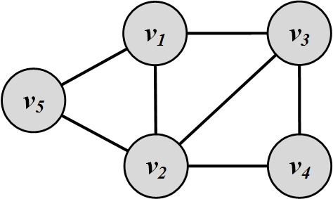
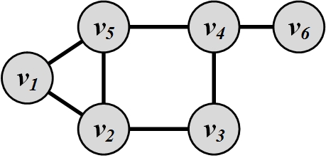
   Example 10.1

   For the graph depicted in Figure 10.5, the similarity between nodes 5 and 7 based on different neighborhood-based techniques is

   

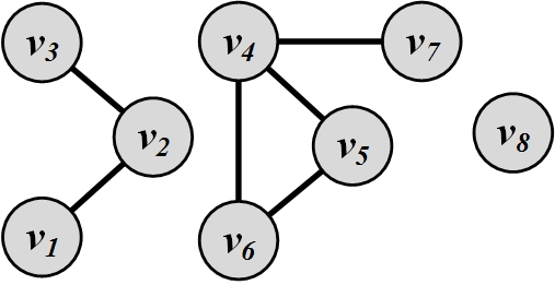
   \text{(Common Neighbor) }\sigma(5,7)= |\{4,6\} \cap \{4\}|=1(10.9)

   \text{(Jaccard) }\sigma(5,7)= \frac{|\{4,6\} \cap \{4\}|}{|\{4,6\} \cup \{4\}|}=\frac{1}{2}(10.10)

   \text{(Adamic and Adar) }\sigma(5,7)= \frac{1}{\log |\{5,6,7\}|}= \frac{1}{\log 3}(10.11)

   \text{(Preferential Attachment) }\sigma(5,7)= |\{4\}|\cdot|\{4,6\}|=1\times 2=2(10.12)

   In Figure 10.5, there are 8 nodes; therefore, we can have a maximum of {8 \choose 2}=28 edges. We already have 6 edges in the graph; hence, there are 28-6=22 other edges that are not in the graph. For all these edges, we can compute the similarity between their endpoints using the aforementioned neighborhood-based techniques and identify the top 3 most likely edges that are going to appear in the graph based on each technique. Table 1.1 shows the top 3 edges based on each technique and the corresponding values for each edge. As shown in this table, different methods predict different edges to be most important; therefore, the method of choice depends on the application.

   Table 10.1: A Comparison between Link Prediction Methods

   	\mathbf{1^{st}~edge}	\mathbf{2^{nd}~edge}	\mathbf{3^{rd}~edge}
   Common Neighbors	\sigma(6,7)=1	\sigma(1,3)=1	\sigma(5,7)=1
   Jaccard Similarity	\sigma(1,3)=1	\sigma(6,7)=1/2	\sigma(5,7)=1/2
   Adamic and Adar	\sigma(1,3)=1/\log 2	\sigma(6,7)=1/\log 3	\sigma(5,7)=1/\log 3
   Preferential Attachment	\sigma(2,4)=6	\sigma(2,5)=4	\sigma(2,6)=4

2. Methods based on paths between nodes. Similarity between nodes can simply be computed from the shortest path distance between them. The closer the nodes are, the higher their similarity. This similarity measure can be extended by considering multiple paths between nodes and their neighbors. The following measures can be used to calculate similarity.

   1. Katz measure. Similar to Katz centrality defined in Chapter 3, one can define the similarity between nodes x and y as

      \sigma(x,y)=\sum_{l=1}^\infty \beta^l |{paths}_{x,y}^{<l>}|,(10.13)

      where |{paths}_{x,y}^{<l>}| denotes the number of paths of length l between x and y. \beta is a constant that exponentially damps longer paths. Note that a very small \beta results in a common neighbor measure (see Exercises). Similar to our finding in Chapter 3, one can find the Katz similarity measure in a closed form by (I-\beta A)^{-1}-I. Katz measure can also be weighted or unweighted. In the unweighted format, |{paths}_{x,y}^{<1>}|=1 if there is an edge between x and y. The weighted graph is more suitable for multigraphs, where multiple edges can exist between the same pair of nodes. For example, consider two authors x and y that have collaborated c times. In this case, |paths_{x,y}^{<1>}|=c.

   2. Hitting and Commute Time. Consider a random walk that starts at node x and moves to adjacent nodes uniformly. Hitting time H_{x,y} is the expected number of random walk steps needed to reach y starting from x. This is a distance measure. In fact, a smaller hitting time implies a higher similarity; therefore, a negation can turn it into a similarity measure.

      \sigma(x,y)= -H_{x,y}.(10.14)

      Note that if node y is highly connected to other nodes in the network, i.e., has a high stationary probability \pi_y, then a random walk starting from any x likely ends up visiting y early. Hence, all hitting times to y are very short and all nodes become similar to y. To account for this, one can normalize hitting time by multiplying it with the stationary probability \pi_y,

      \sigma(x,y)= -H_{x,y}\pi_y.(10.15)

      Hitting time is not symmetric and in general, H_{x,y}\neq H_{y,x}. Thus, one can introduce the commute time to mitigate this issue,

      \sigma(x,y)= -(H_{x,y}+H_{y,x}).(10.16)

      Similarly, commute time can also be normalized,

      \sigma(x,y)= -(H_{x,y}\pi_y+H_{y,x}\pi_x).(10.17)

   3. Rooted PageRank. A modified version of the PageRank algorithm can be used to measure similarity between two nodes x and y. In rooted PageRank, we measure the stationary probability of y: \pi_y given the condition that during each random walk step, we jump to x with probability \alpha or a random neighbor with probability 1-\alpha. Matrix format discussed in Chapter 3 can be used to solve this problem.

   4. SimRank. One can define similarity between two nodes recursively based on the similarity between their neighbors. In other words, similar nodes have similar neighbors. SimRank performs the following:

      \sigma(x,y)= \gamma. \frac{\sum_{x' \in N(x)}\sum_{y' \in N(y)}\sigma(x',y')}{|N(x)||N(y)|},(10.18)

      where \gamma is some value in range [0,1]. We set \sigma(x,x)=1 and by finding the fixed point of this equation, we can find the similarity between node x and node y

After one of the aforementioned measures is selected, a list of top most similar pairs of nodes are selected. These pairs of nodes denote edges predicted to be the most likely to soon appear in the network. Performance (precision, recall, or accuracy) can be evaluated using the testing graph and by comparing the number of the testing graph’s edges the link prediction algorithm successfully reveals. Note that the performance is usually very low, since many edges are created due to reasons not solely available in a social network graph. So, a common baseline is to compare the performance with random edge predictors and report the factor improvements over random prediction.

10.2 Collective Behavior

Collective behavior, first defined by sociologist Robert Park, refers to a population of individuals behaving in a similar way. This similar behavior can be planned and coordinated, but is often spontaneous and without any plans. For instance, individuals stand in line for a new product release, rush into stores for a sale event, and post messages online to support their cause or show their support for an individual. These events, though formed by independent individuals, are observed as a collective behavior by outsiders.

10.2.1 Collective Behavior Analysis

Collective behavior analysis is often performed by analyzing individuals performing the behavior. In other words, one can divide collective behavior into many individual behaviors and analyze them independently. The result, however, would be an expected behavior for a large population when all these analyses are put together. The user migration behavior we discussed in this section is an example of such analysis of collective behavior.

One can also analyze the population as a whole. In this case, an individual’s opinion or behavior is rarely important. In general, the approach is the same as analyzing an individual, with the difference that the content and links are now considered for a large community. For instance, if we are analyzing 1,000 nodes one can combine these nodes and edges into one hyper-node, where the hyper-node is connected to all other nodes in the graph to which its members are connected to and has an internal structure (subgraph) that details the interaction among its members. This approach is unpopular for analyzing collective behavior. Interested readers can refer to bibliographic notes for further references that utilize this approach to analyze collective behavior. On the contrary, this approach is often considered when predicting collective behavior, which will be discussed later in this chapter.

User Migration in Social Media

Users often migrate from one site to another for different reasons. The main rationale behind it is that users have to select some sites over others due to their limited time and resources. Moreover, social media’s networking often dictates that one cannot freely choose a site to join or stay. An individual’s decision is heavily influenced by her friends, and vice versa. Ultimately, this entails user migrations. Sites are often interested in keeping their users, as they are valuable assets for the site and help contribute to the growth of a site and generate revenue by increased traffic. There are two types of migration that take place in social media sites: site migration and attention migration.

• Site Migration. For any user that is a member of two sites s_1 and s_2 at time t_i, and is only left member of s_2 at time t_j>t_i, then the user is said to have migrated from site s_1 to site s_2.

• Attention Migration. For any user that is a member of two sites s_1 and s_2 and is active at both at time t_i, if the user becomes inactive on s_1 and remains active on s_2 at time t_j>t_i, then the user’s attention is said to have migrated away from site s_1 and towards site s_2.

Activity (or inactivity) of a user can be determined by observing the user’s actions performed on the site. For instance, we can consider a user active in interval [t_i,t_i+\delta], if the user has performed at least one action on the site during this interval. Otherwise, the user is considered inactive.

The interval \delta could be measured at different granularity, such as days, weeks, months, and years. To measure user activity, it is common to set \delta=1 month. To analyze the migration of populations across sites, we can analyze migrations of individuals and then measure the rate at which the population of these individuals is migrating across sites. Since we analyze migrations at the individual’s level, we can utilize the methodology outlined in Section 1.1.1.2 for individual behavior analysis as follows:

1. The observable behavior. Site migration is rarely observed since users often abandon their accounts rather than closing them. A more observable behavior is attention migration, which is clearly observable on most social media sites. Moreover, when a user commits site migration, it is often too late to perform preventive measures. However, when attention migration is detected, it is still possible to take actions to retain the user or expedite his attention migration to guarantee site migration. Thus, we focus on individuals whose attention has migrated.

   To observe attention migrations, several steps need to be taken. First, users are required to be identified on multiple networks so that their activity on multiple sites can be monitored simultaneously. For instance, username huan.liu1 on Facebook is username liuhuan on Twitter. This can be done by collecting information from sites where individuals list their multiple identities on social media sites. On social networking sites such as Google+ or Facebook, this happens regularly. The second step is collecting multiple snapshots of social media sites. At least two snapshots are required to observe migrations. After these two steps, we can observe whether attention migrations have taken place or not. In other words, we can observe if users have become inactive on one of the sites over time. Figure 10.6 depicts these migrations for some well-known social media sites. In this figure, each radarchart shows migrations from a site to multiple sites. Each target site is shown as a vertex and the longer the spokes towards that site, the larger the migrating population to it.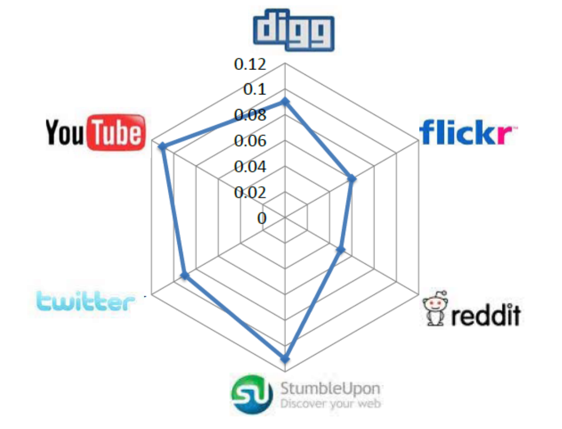

   

   (a) Delicious

   

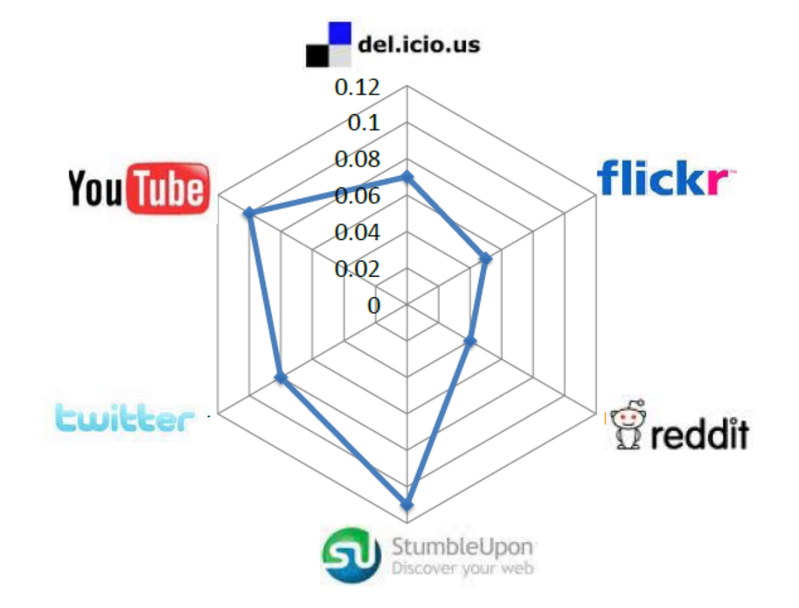   (b) Digg

   

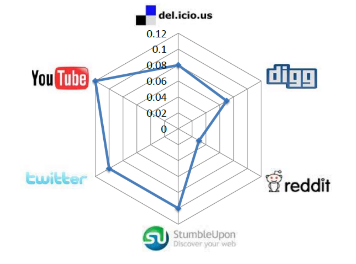   (c) Flickr

   

   (d) Reddit

   

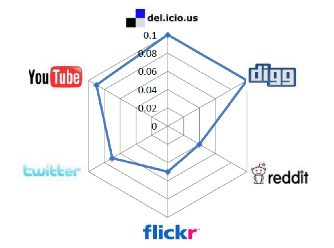   (e) StumbleUpon

   

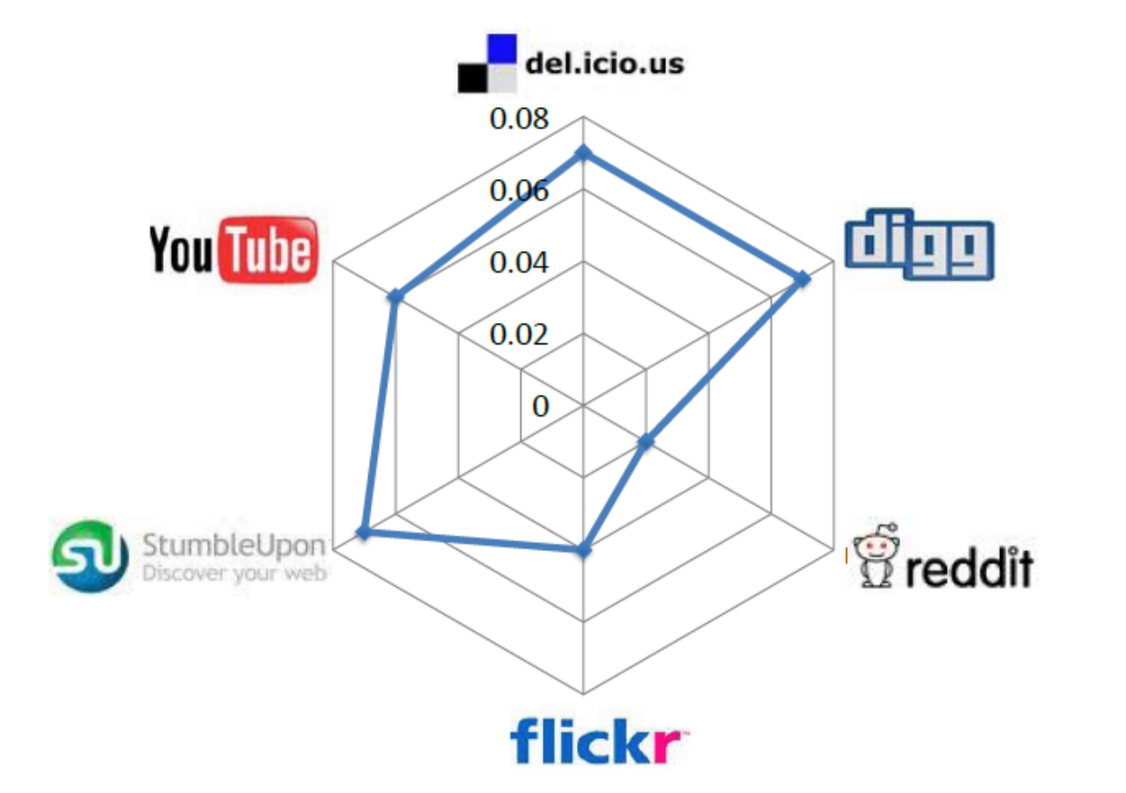   (f) Twitter

   

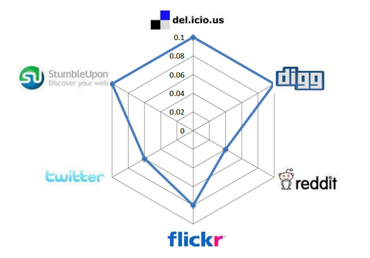   (g) YouTube

2. Features. Three general features can be considered for user migration. These are 1) user activity on one site, 2) user network size, and 3) user rank. User activity is important, since we can conjecture that a more active user on one site is less likely to migrate. User network size is important, since a user with more social ties (i.e., friends) in a social network is less probable to move. Finally, user rank is important. The rank is the value of a user as perceived by others. A user with high status in a network is less likely to move to a new one where he or she must spend more time getting established.

   User activity can be measured differently for different sites. On Twitter, this can be the number of tweets posted by the user, on Flickr, the number photos uploaded by the user, and on Youtube, the number of videos the user has uploaded. One can normalize this value by its maximum in the site (e.g., the maximum number of videos any user has uploaded) to get an activity measure in the range [0,1]. If a user is allowed to have multiple activities on a site, as in posting comments and liking videos, then a linear combination of these measures can be used to describe user activity on a site.

   User network size can be easily measured by taking the number of friends a user has osn the site. It is common for social media sites to facilitate adding friends. The number of friends can be normalized in the range [0,1] by the maximum number of friends on the site.

   Finally, user rank is how important a user is on the site. Some sites explicitly provide their users’ prestige rank list (e.g., top 100 bloggers), while for others, one needs to approximate a user’s rank. One way of approximating it is to count the number of citations (in-links) an individual is receiving from others. A practical technique is to perform this via web search engines. For instance, user test on StumbleUpon will have http://test.stumpleupon.com as his profile page. A Google search for link:http://test.stumbleupon.com provides us with the number of in-links to the profile on StumbleUpon and can be considered as a ranking measure for user test.

   These three features are correlated with the site attention migration behavior and one expects changes in them when migrations happen.

3. Feature-Behavior Association. Given two snapshots of a network, we know if users migrated or not. We can also compute the values for the aforementioned features. Hence, we can determine the correlation between features and migration behavior.

   Let vector Y \in \mathbb{R}^n indicate whether any of our n users have migrated or not. Let X_t \in \mathbb{R}^{3\times n} be the features collected (activity, friends, rank) for any one of these users at time stamp t. Then, the correlation between features X and labels Y can be computed via logistic regression. How can we verify that this correlation is not random? Next, we discuss how we verify that this correlation is statistically significant.

4. Evaluation Strategy. To verify if the correlation between features and the migration behavior is not random, we can construct a random set of migrating users and compute X_{Random} and Y_{Random} for them, as well. This can be obtained by shuffling the original X and Y. Then, we perform logistic regression on these new variables. This approach is very similar to the shuffle test presented in Chapter 8. The idea is that if some behavior creates a change in features, then other random behaviors should not create that drastic a change. So, the observed correlation between features and the behavior should be significantly different in both cases. The correlation can be described in terms of logistic regression coefficients and the significance can be measured via any significance testing methodology. For instance, we can employ \chi^2-statistic

   \chi^2-statistic,

   \chi^2 = \sum_{i=1}^{n} \frac{(A_i - R_i)^2}{R_i},(10.19)

   where n is the number of logistic regression coefficients, A_i’s are the coefficients determined using the original dataset, and R_i’s are the coefficients obtained from the random dataset.

10.2.2 Collective Behavior Modeling

Consider a hypothetical model than can simulate voters who cast ballots in elections. This effective model can help predict an election’s turnout rate as an outcome of the collective behavior of voting and help governments prepare logistics accordingly. This is an example of collective behavior modeling. Similar to individual behavior modeling, collective behavior modeling improves our understanding of the collective behaviors that take place by providing concrete explanations.

Collective behavior can be conveniently modeled using some of the techniques discussed in Network Models (Chapter 4). Similar to collective behavior, in network models, we express models in terms of characteristics observable in the population. For instance, when having power-law degree distribution is required, the preferential attachment model is preferred, and when small average shortest path is desired, the small-world model is the method of choice. In network models, node properties rarely play a role; therefore, they are reasonable for modeling collective behavior.

10.2.3 Collective Behavior Prediction

Collective behavior can be predicted using methods we discussed in Chapters 7 and 8. For instance, epidemics can predict the effect of a disease on a population and the behavior that the population will exhibit over time. Similarly, implicit influence models such as the LIM model discussed in Chapter 8 can estimate influence of individuals based on collective behavior attributes, such as the size of the population adapting an innovation at any time.

As noted before, collective behavior can be analyzed either in terms of individuals forming the collective behavior or using the population as a whole. When predicting collective behavior, it is common to consider the population as a whole and aim at predicting some phenomenon. This simplifies the challenges and reduces the computation dramatically, since the number of individuals that form a collective behavior is often large and analyzing them one at a time is cumbersome.

In general, when predicting collective behavior, we are interested in predicting the intensity of a phenomenon, which is due to the collective behavior of the population, e.g., how many of them will vote? To perform this prediction, we utilize a data mining approach where features that describe the population well are utilized to predict a response variable, i.e., the intensity of the phenomenon. A training-testing framework or correlation analysis is used to determine the generalization and the accuracy of the predictions. We discuss This collective behavior prediction strategy through the following example. This example demonstrates how the collective behavior of individuals on social media can be utilized to predict real-world outcomes.

Predicting Box-Office Revenue for Movies

Can we predict opening-weekend revenue for a movie from its pre-release chatter among fans? This tempting goal of predicting the future has been around for many years. The goal is to predict the collective behavior of watching a movie by a large population, which in turn results in the revenue for the movie. One can design a methodology to predict box-office revenue for movies utilizing Twitter and using the aforementioned collective behavior prediction strategy. To summarize, the strategy is as follows:

1. Set the target variable which is being predicted. In this case, it is the revenue that a movie produces. Note that the revenue is the direct result of the collective behavior of going to the theater to watch the movie.

2. Determine the feature in the population that may affect the target variable.

3. Predict the target variable using a supervised learning approach, utilizing the features.

4. Measure performance using supervised learning evaluation.

One can utilize the population that is discussing the movie on Twitter before its release to predict its opening-weekend revenue. The target variable is the amount of revenue. In fact, utilizing only 8 features, one can predict the revenue with high accuracy. These features are the average hourly number of tweets related to the movie for each of the 7 days prior to the movie opening (7 features) and the number of opening theaters for the movie (1 feature). Using only these 8 features, training data for some movies (their 7 day tweet rates and the revenue), and a linear regression model, one can predict the movie opening-weekend revenue with high correlation. It has been shown by researchers (see bibliographic notes) that the predictions using this approach are closer to reality than that of the Hollywood Stock Exchange (HSX), which is the gold standard for predicting revenues for movies.

This simple model for predicting movie revenue can be easily extended to other domains. For instance, assume we are planning to predict another collective behavior outcome, such as the number of individuals that aim to buy a product. In this case, the target variable y is the number of individuals that will buy the product. Similar to tweet rate, we require some feature A that denotes the attention the product is receiving. We also need to model the publicity of the product P. In our example, this was the number of theaters for the movie, and for products, it could represent the number of stores that sell the product. A simple linear regression model can help learn the relation between these features and the target variable:

where \epsilon is the regression error. Similar to our movie example, one attempts to extract the values for A and P from social media.

10.3 Summary

Individuals exhibit different behaviors on social media, which can be categorized into individual and collective behavior. Individual behavior is the behavior that an individual targets toward 1) another individual (individual-individual behavior), 2) an entity (individual-entity behavior), or 3) a community (individual-community behavior). We discuss how to analyze and predict individual behavior. To analyze individual behavior, a four-step procedure is outlined as guideline. First, the behavior observed should be clearly observable on social media. Second, one needs to design meaningful features that are correlated with the behavior taking place in social media. The third step aims at finding correlations and relationships between features and the behavior. The final step is to verify these relationships found. We discuss community joining as an example of individual behavior. Modeling individual behavior can be performed via cascade or threshold models. Behaviors commonly result in interactions in the form of links; therefore, link prediction techniques are highly efficient in predicting behavior. We discuss neighborhood-based and path-based techniques for link prediction.

Collective behavior is when a group of individuals with or without coordination act in an aligned manner. Collective behavior analysis is either done via individual behavior analysis and then averaged or analyzed collectively. When analyzed collectively, one commonly looks at the general patterns of the population. We discuss user migrations in social media as an example for collective behavior analysis. Modeling collective behavior can be performed via network models and prediction is possible by utilizing population properties to predict an outcome. Predicting movie box-office revenues is given as an example, which uses population properties such as the rate at which they are tweeting to demonstrate the effectiveness of this approach.

It is important to evaluate behavior analytics findings to ensure that these finding are not due to externalities. We discuss causality testing, randomization tests, and supervised learning evaluation techniques for evaluating behavior analytics finding. However, depending on the context, researchers may need to devise other informative techniques to ensure the validity of the outcomes.

10.4 Bibliographic Notes

In addition to methods discussed in this chapter, game theory and theories from economics can be utilized to analyze human behavior (Easley and Kleinberg 2010). Community joining behavior analysis was first introduced by Backstrom et al. (Backstrom et al. 2006). The approach discussed in this chapter is a brief summary of their approach for analyzing community joining behavior. Among other individual behaviors, tie formation is analyzed in detail. In (Wang et al. 2010), the authors analyze tie formation behavior on Facebook and investigate how visual cues influence individuals with no prior interaction to form ties. The features used are gender, i.e., male or female, and visual conditions (attractive, non-attractive, and no photo). Their analyses show that individuals have a tendency to connect to attractive opposite-sex individuals when no other information is available. Analyzing individual information sharing behavior helps understand how individuals disseminate information on social media. Gundecha et al. (Gundecha et al. 2011) analyze how the information sharing behavior of individuals result in vulnerabilties and how one can exploit such vulnerabilities to secure user privacy on a social networking site. Finally, most social media mining research is dedicated to analyzing a single site; however, users are often members of different sites and hence, current studies need to be generalized to cover multiple sites. Zafarani et. al (Zafarani and Liu 2013, 2009) were the first to design methods that help connect user identities across social media sites using behavioral modeling. A study of user tagging behavior across sites is available in (Wang et al. 2011).

General surveys on link prediction can be found in (Adamic and Adar 2003; Liben-Nowell and Kleinberg 2007; Al Hasan et al. 2006; Lü and Zhou 2011). Individual behavior prediction is an active area of research. Location prediction is an active area of individual behavior widely studied over a long period in the realm of mobile computing. Researchers analyze human mobility patterns to improve location prediction services, and therefore exploit their potential power on various applications such as mobile marketing (Barnes and Scornavacca 2004; Barwise and Strong 2002), traffic planning (Ben-Akiva et al. 1998; Dia 2001), and even disaster relief (H. Gao et al. 2011, 2012a; Goodchild and Glennon 2010; Wang and Huang 2010; Huiji Gao et al. 2011; Barbier et al. 2012; Kumar et al. 2013). Other general references can be found in (Backstrom et al. 2010; Monreale et al. 2009; Spaccapietra et al. 2008; Thanh and Phuong 2007; Scellato et al. 2011; H. Gao et al. 2012b; Huiji Gao et al. 2012).

Kumar et al. (Kumar et al. 2011) first analyzed migration in social media. Other collective behavior analyses can be found in (Leskovec et al. 2009). The movie revenue prediction was first discussed by Asur and Huberman (Asur and Huberman 2010). Another example of collective behavior prediction can be found in the work of O’Connor et al. (O’Connor et al. 2010), which proposed using Twitter data for opinion polls. Their results are highly correlated with Gallup opinion polls for presidential job approval. In (Abbasi et al. 2012), Abbasi et al. analyzed collective social media data and show that by carefully selecting data from social media, it is possible to use social media as a lens to analyze and even predict real-world events.