Community Analysis
In November 2010, the authorities dismantled a community of 30 million infected computers across the globe that were sending more than 3.6 billion daily spam-mails. These distributed networks of infected computers are called botnets. The community of computers in a botnet are transmitting spam or viruses across the web without their owner’s permission. The members of a botnet are rarely known; however, it is vital to identify these botnet communities and analyze their behavior to enhance internet security. This is an example of community analysis. In this chapter, we discuss community analysis in social media.
Also known as groups, clusters, or cohesive subgroups, communities have been studied extensively in many fields and in particular, social sciences. In social media mining, analyzing communities is essential. The importance of studying communities in social media is multi-fold. First, individuals often form groups based on their interests and when studying individuals, we are interested in identifying these groups. Consider the importance of finding groups with similar reading tastes by an online book seller for recommendation purposes. Second, groups provide a clear global-view of user interactions, whereas a local-view of individual behavior is often noisy and ad hoc. Finally, specific behaviors are only observable in a group setting and not on an individual level. This is because the individual’s behavior can fluctuate, but the group collective behavior is more robust to change. Consider the interactions between two opposing political groups on social media. Two individuals, one from each group, can hold similar opinions on a debating subject, but what is important is that their communities can exhibit opposing views on the same subject.
In this chapter, we discuss communities and answer the following questions in detail:
How can we detect communities? This question is discussed in different sciences, but in diverse forms. In particular, quantization in electrical engineering, discretization in statistics, or clustering in machine learning tackle a similar challenge. As discussed in Chapter 5, in clustering, data points are grouped together based on a similarity measure. In community detection, data points represent actors in social media and similarity between these actors is often defined based on the interests these users share. The major difference between clustering and community detection is that in community detection, individuals are connected to others via a network of links, whereas in clustering, data points are not embedded in a network.
How do communities evolve and how can we study evolving communities? Social media is a dynamic and evolving environment. Similar to real-world friendships, social media interactions evolve over time. People join or leave groups and groups expand, shrink, dissolve, or split over time. Studying temporal behavior of communities is necessary for a deep understanding of communities in social media.
How can we evaluate detected communities? As emphasized in our botnet example, the list of community members (i.e., ground truth) is rarely known. Hence, community evaluation is a challenging task and is often translated to evaluating detected communities in the absence of ground truth.
6.0.1 Social Communities
Broadly speaking, a real-world community is a body of individuals with common economic, social, or political interests/characteristics, often living in relative proximity. A trivial community comes to existence when like-minded users on social media form a link and start interacting with each other. In other words, any formation of a community requires 1) a set of at least two nodes sharing some interest and 2) interactions with respect to that interest.
As a real-world community example, consider the famous example of a college karate club interactions collected by Wayne Zachary in 1977. The example is often referred to as Zachary’s Karate Club
Zachary’s Karate Club(Zachary 1977) in the literature. Figure 6.1 depicts the interactions in a college karate club over 2 years. Links demonstrate friendships between members. During the observation period, individuals split into two communities due to disagreement between the club administrator and the karate instructor and members of one community left to start their own club. In this figure, node colors demonstrate the communities individuals belong to. As observed in this figure, utilizing graphs is a convenient way for depicting communities as color-coding nodes allows to denote memberships and edges can be used to denote relations. Furthermore, we can observe that individuals are more likely to be friends with members of their own group, hence, creating tightly-knit components in the graph.
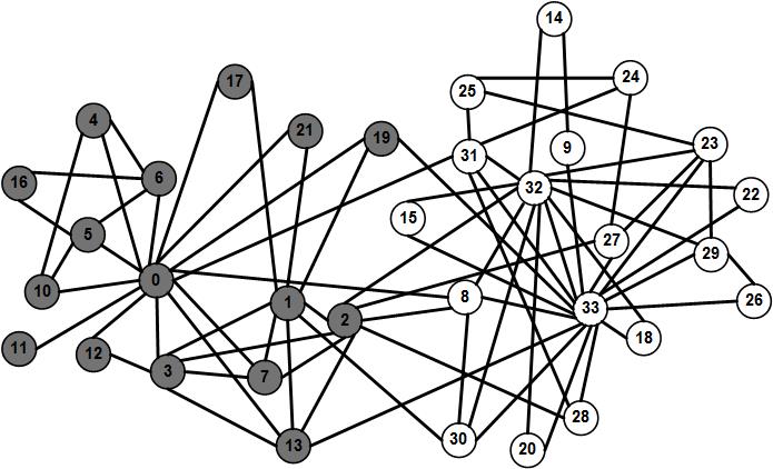
Zachary’s Karate club is an example of two explicit communities
Explicit (emic)
Communities. An explicit community, also known as an emic community, is one where
Community members understand that they are its members;
Non-members understand who the community members are; and
Community members often have more interactions with each other than non-members.
In contrast to explicit communities, in implicit communities
Implicit (etic)
Communities, also known as etic communities, one is tacitly interacting with others in the form of an unacknowledged community. For instance, individuals calling Canada from the United States on a daily basis need not be friends and don’t consider one another as members of the same explicit community. However, from the phone operator’s point of view, they form an implicit community that needs to be marketed the same promotions. Finding implicit communities is of major interest and this chapter aims at finding these communities in social media.
Communities in social media are more or less representatives of communities in real-world. As mentioned, in real-world, communities are commonly geographically close. The geographical location becomes less important when in social media and many communities on social media consist of highly diverse people from all around the planet. In general, people in real-world communities tend to be more similar than those of social media. People do not need to share language, location, etc. to be members of social media communities. Similar to real-world communities, communities in social media can be labeled as explicit or implicit. As examples of explicit communities in well-known social media sites, consider
Facebook. In Facebook, there exist a variety of explicit communities, such as groups, communities, among others. In these communities, users can post messages and images, comment on other messages, like posts, and view activities of others.
Yahoo! Groups. In Yahoo! groups, individuals join a group mailing list where they can receive emails from all or a selection of group members (administrators) directly.
LinkedIn. LinkedIn provides its users with a feature called Groups and Associations. Users can join professional groups where they can post and share information related to the group.
As these represent explicit communities, individuals have an understanding of when they are joining them. However, there exist implicit communities in social media as well. For instance, consider individuals with the same taste for certain movie on a movie rental site. These individuals are rarely all members of the same explicit community. However, the movie rental site is particularly interested in finding these implicit communities since it can better market to them by recommending movies similar to their tastes. We discuss techniques to find these implicit communities next.
6.1 Community Detection
As mentioned earlier, communities can be explicit (e.g., Yahoo! groups), or implicit (e.g., individuals who write blogs on the same or similar topics). In contrast to explicit communities, in many social media sites, implicit communities and their members are obscure to many. Community detection finds these implicit communities.
In its simplest form, similar to the graph shown in Figure 6.1, community detection algorithms are often provided with a graph where nodes represent individuals and edges represent friendship between individual. This definition can be generalized. Edges can also be used to represent contents or attributes shared by individuals. For instance, we can connect individuals at the same location, with the same gender, or who bought the same product using edges. Similarly, nodes can also represent products, sites, and webpages, among others. Formally, for a graph G(V,E), the task of community detection is to find a set of communities \{C_i\}_{i=1}^n in a G such that \cup_{i=1}^n C_i \subseteq V.
6.1.1 Community Detection Algorithms
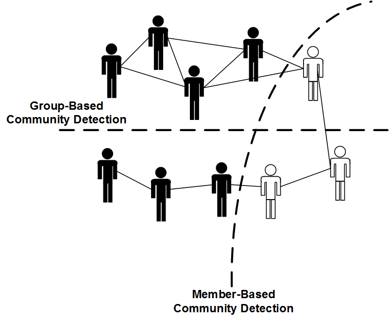
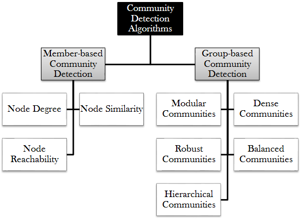
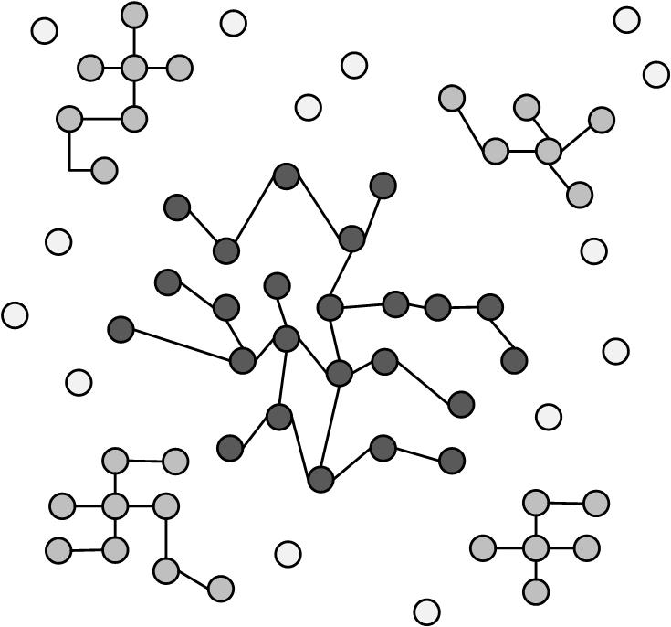
There is a variety of community detection algorithms. When detecting communities, we are either interested in detecting communities with 1) specific members or 2) specific forms of communities. We denote the former as member-based community detection and the latter as group-based community detection. Consider the network of 10 individuals shown in Figure 6.2 where 7 are wearing black t-shirts and 3 are wearing white ones. If we group individuals based on their t-shirt color, we end up having a community of 3 and a community of 7. This is an example of member-based community detection, where we are interested in specific members characterized by their t-shirts’ color. If we group the same set based on the density of interactions (i.e., internal edges), we get two other communities. This is an instance of group-based community detection, where we are interested in specific communities characterized by their interactions’ density.
In member-based community detection, we introduce community detection algorithms that group members based on attributes or measures such as similarity, degree, or reachability. In group-based community detection, we are interested in finding communities that are modular, balanced, dense, robust, or hierarchical.
6.1.2 Member-based Community Detection
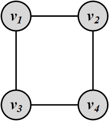
The intuition behind member-based community detection is that members with the same (or similar) characteristics are more often in the same community. Therefore, a community detection algorithm following this approach should assign members with similar characteristics to the same community. Let us consider a simple example. We can assume nodes that belong to a cycle form a community. This is because they share the same characteristic: being in the cycle. Figure 6.3 depicts a 4-cycle. For instance, we can search for all n-cycles in the graph and assume that they represent a community. The choice for n can be based on empirical evidence or heuristics or n can be in a range [\alpha_1, \alpha_2] for which all cycles are found. A well-known example is the search for 3-cycles (triads) in graphs.
In theory, any subgraph can be searched for and assumed to be a community. In practice, only subgraphs that have nodes with specific characteristics are considered as communities. Three general node characteristics that are frequently used are: node similarity, node degree (familiarity), and node reachibility.
When employing node degrees, we seek subgraphs, often connected, such that each node (or a subset of nodes) has a certain node degree (number of incoming or outgoing edges). Our 4-cycle example follows this property, the degree of each node being two. In reachability, we seek subgraphs with specific properties related to paths existing between nodes. For instance, our 4-cycle instance also follows the reachability characteristic where all pairs of nodes can be reached via two independent paths. In node similarity, we assume nodes that are highly similar belong to the same community.
Node Degree
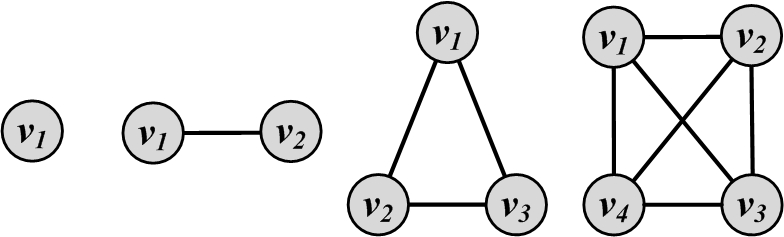
The most common subgraph searched for in networks based on node degrees is clique. A clique is a maximum complete subgraph in which all pairs of nodes are connected. In terms of degree characteristic, a clique of size k is a subgraph of k nodes where all node degrees are k-1. The only difference between cliques and complete graphs is that cliques are subgraphs, whereas complete graphs contain the whole node set V. The simplest four complete graphs (or cliques, when these are subgraphs) are represented in Figure 6.4.
To find communities, we can search for the maximum clique (the one with the largest number of vertices) or all maximal cliques (cliques that are not subgraphs of a larger clique, i.e., cannot be further expanded). However, both problems are NP-hard, as is verifying whether a graph contains a clique larger than size k. To overcome these theoretical barriers, for sufficiently small networks or subgraphs, we can 1) use brute-force, 2) add some constraints such that the problem is relaxed and polynomially solvable, or 3) use cliques as the seed or core of a larger community.
Brute-force clique identification. The brute force method can find all maximal cliques in a graph. For each vertex v_x, we try to find the maximal clique that contains node v_x. The brute-force algorithm is detailed in Algorithm 6.1.
- Require: Adjacency Matrix A, Vertex v_x
- return Maximal Clique C containing v_x
- CliqueQueue = \{\{v_x\}\};
- while CliqueQueue has not changed do
- C=pop(CliqueQueue);
- v_{last} = Last node added to C;
- N(v_{last})=\{v_i|A_{v_{last},v_i}=1\}.
- for all v_{temp} \in N(v_{last}) do
- if C \bigcup \{v_{temp}\} is a clique then
- push(CliqueQueue, C \bigcup \{v_{temp}\});
- end if
- end for
- end while
- Return the largest clique from CliqueQueue
The algorithm starts with an empty queue of cliques. This queue is initialized with the node v_x that is being analyzed (a clique of size 1). Then, from the queue, a clique is popped (C). The last node added to clique C is selected (v_{last}). All the neighbors of v_{last} are added to the popped clique C sequentially and if the new set of nodes creates a larger clique (i.e., the newly added node is connected to all of the other members), then the new clique is pushed back into the queue. This procedure is followed until nodes can no longer be added.
The brute-force algorithm becomes impractical for large networks. For instance, for a complete graph of only 100 nodes, the algorithm will generate 2^{100} different cliques starting from any node in the graph (why?).
The performance of the brute-force algorithm can be enhanced by pruning specific nodes and edges. If the cliques being searched for are of size k or larger, we can simply assume that the clique, if found, should contain nodes that have degrees equal to or more than k-1. We can first prune all nodes (and edges connected to them) with degrees less than k-1. Due to powerlaw distribution of node degrees, many nodes exist with small degrees (1, 2, etc.). Hence, for a large enough k many nodes and edges will be pruned, which will reduce the computation drastically. This pruning works for both directed and undirected graphs.
Even with pruning, there are intrinsic properties with cliques that make them a less desirable means for finding communities. Cliques are rarely observed in real-world. For instance, consider a clique of 1,000 nodes. This subgraph has \frac{99 \times 1000}{2}=499,500 edges. A single edge removal from this many edges results in a subgraph which is no longer a clique. That is less than 0.0002% of the edges. This makes finding cliques an unlikely and challenging task.
In practice, to overcome this challenge, we can either relax the clique structure or use cliques as a seed or core of a community.
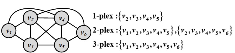
Relaxing Cliques. A well-known clique relaxation that comes from sociology is the k-plex concept
k-plex. In a clique of size k, all nodes have the degree of k-1; however, in a k-plex, all nodes have a minimum degree that is not necessarily k-1 (as opposed to cliques of size k). For a set of vertices V, the structure is called a k-plex if we have,
Clearly, a clique of size k is a 1-plex. As k gets larger in a k-plex, the structure gets increasingly relaxed, since we can remove more edges from the clique structure. Finding the maximum k-plex in a graph still tends to be NP-Hard but in practice, finding it is relatively easier due to smaller search space. Figure 6.5 shows k-plexes for k = 1, 2, and 3.
Using Cliques as a Seed of a Community. When using cliques as a seed or core of a community, we assume communities are formed from a set of cliques (small or large) in addition to edges that connect these cliques. A well-know algorithm in this area is the clique percolation method (CPM)
Clique
Percolation
Method (CPM)(Palla et al. 2005). The algorithm is provided in Algorithm 6.2. Given parameter k, the method starts by finding all cliques of size k. Then a graph is generated (clique graph) where all cliques are represented as nodes and cliques that share k-1 vertices are connected via edges. Communities are then found by reporting the connected components of this graph. The algorithm searches for all cliques of size k and is therefore computationally intensive. In practice, when using the CPM algorithm, we often solve CPM for a small k. Relaxations discussed for cliques are desirable for the algorithm to perform faster. Lastly, CPM can return overlapping communities.
- Require: parameter k
- return Overlapping Communities
- {Cliques}_k = find all cliques of size k
- Construct clique graph G(V,E), where |V| = |{Cliques}_k|
- E= {e_{ij} | clique i and clique j share k-1 nodes}
- Return all connected components of G
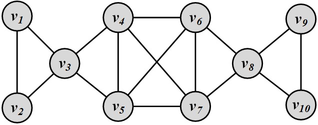
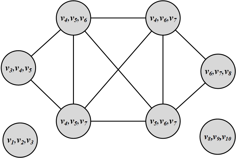
Consider the network depicted in Figure 6.6(a). The corresponding clique graph generated by the CPM algorithm for k=3 is provided in Figure 6.6(b). All cliques of size k=3 have been identified and cliques that share k-1 = 2 nodes are connected. Connected components are returned as communities (\{v_1, v_2, v_3\}, \{v_8, v_9, v_{10}\} and \{v_3, v_4, v_5, v_6, v_7, v_8\}). Nodes v_3 and v_8 belong to two communities and these communities are overlapping.
Node Reachability
When dealing with reachability we are seeking subgraphs where nodes are reachable from other nodes via a path. The two extremes of reachability are achieved when nodes are assumed to be in the same community if 1) there is a path between them (regardless of the distance) or 2) they are so close as to be immediate neighbors. In the first case, any graph traversal algorithm such as BFS or DFS can be used to identify connected components (communities). Finding connected components is not very useful in large social media networks. These networks tend to have a large scale connected component that contains most nodes, which are connected to each other via short paths. Therefore, finding connected components is less powerful for detecting communities in them. In the second case, when nodes are immediate neighbors of all other nodes, cliques are formed and as discussed previously, finding cliques is considered a very unlikely and challenging process.
To overcome these issues, we can find communities that are in between cliques and connected components in terms of connectivity and have small shortest paths between their nodes. There are predefined subgraphs, with roots in social sciences, with these characteristics. Well-known ones include the following:
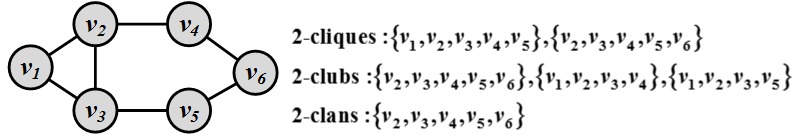
k-Clique, k-Club, and k-Clank-Clique is a maximal subgraph where the shortest path between any two nodes is always less than or equal to k. Note that in k-cliques, nodes on the shortest path should not necessarily be part of the subgraph.
k-Club is a more restricted definition; it follows the same definition as k-cliques with the additional constraint that nodes on the shortest paths should be part of the subgraph.
k-Clan is a k-clique where for all shortest paths within the subgraph, the distance is less than or equal to k. All k-clans are k-cliques and k-clubs, but not vice versa. In other words,
k-Clans = k-Cliques \cap k-Clubs.
Figure 6.7 depicts an example of the three discussed models.
Node Similarity
Node similarity attempts to determine the similarity between two nodes v_i and v_j. Similar nodes (or most similar nodes) are assumed to be in the same community. The question has been answered in different fields; particularly, the problem of
Structural
Equivalencestructural equivalence in the field of sociology considers the same problem. In structural equivalence, similarity is based on the overlap between the neighborhood of the vertices. Let N_i and N_j be the neighbors of vertices v_i and v_j, respectively. In this case, a measure of vertex similarity can be defined as follows:
For large networks, this value can increase rapidly, since nodes may share many neighbors. Generally, similarity is attributed to a value that is bounded and usually in the range [0,1]. For that to happen, various normalization procedures such as the Jaccard similarity or the Cosine similarity can take place:
Consider the graph in Figure 6.7. The similarity values between nodes 2 and 5 are
In general, the definition of neighborhood N_i excludes the node itself (v_i). This, however, leads to problems with the aforementioned similarities because nodes that are connected and do not share a neighbor will be assigned zero similarity. This can be rectified by assuming that nodes are included in their own neighborhood.
A generalization of structural equivalence is known as regular equivalence. Consider the situation of two basketball players in two different countries. Though sharing no neighborhood overlap, the social circles of these players (coach, players, fans, etc.) might look quite similar due to their social status. In other words, nodes are regularly equivalent when they are connected to nodes that are themselves similar (a self-referential definition). For more details on Regular Equivalence, refer to Chapter 3.
6.1.3 Group-based Community Detection
When considering community characteristics for community detection, we are interested in communities that have certain group properties. In this section, we discuss communities that are balanced, robust, modular, dense, or hierarchical.
Balanced Communities
As mentioned before, community detection can be thought as the problem of clustering in data mining and machine learning. Graph-based clustering techniques have proven to be useful in identifying communities in social networks. In graph-based clustering, we cut the graph into several partitions and assume these partitions represent communities.
Formally, a cut in a graph is a partitioning (cut) of the graph into two (or more) sets (cutsets). The size of the cut is the number of edges that are being cut and the summation of weights of edges that are being cut in a weighted graph. A minimum cut (min-cut) is a cut such that the size of the cut is minimized. Figure 6.8 depicts several cuts in a graph. For example, cut B has size 4 and A is the minimum cut
Minimum Cut.
Based on the well-known max-flow min-cut theorem, the minimum cut of a graph can be computed efficiently.
However, minimum cuts are not always preferred for community detection. Often, minimum cuts result in cuts where a partition is only one node (singleton) and the rest of the graph is in the other. Typically, communities with balanced sizes are preferred. Figure 6.8 depicts an example where the minimum cut (A) creates unbalanced partitions, whereas, cut C is a more balanced cut.
To solve this problem, variants of minimum cut define an objective function, minimizing (or maximizing) which during cut finding procedure, results in a more balanced and natural partitioning of the data. Consider a graph G(V,E). A partitioning of G into k partitions is a tuple P=(P_1, P_2, P_3, \dots, P_k), such that P_i \subseteq V, P_i \cap P_j = \emptyset and \bigcup_{i=1}^{k} P_i = V. Then, the objective function for ratio and normalized cut
Ratio cut and
Normalized Cutare defined as follows:
where \bar{P}_i=V-P_i is the complement cut set, cut(P_i, \bar{P}_i) is the size of the cut, and volume vol(P_i) = \sum_{v \in P_i} d_v. Both objective functions provide a more balanced community size by normalizing the cut size either by the number of vertices in the cutset or the volume (total degree).
Both ratio cut and normalized cut can be formulated in a matrix format. Let matrix X \in \{0,1\}^{|V|\times k} denote the community membership matrix, where X_{i,j}=1 if node i is in community j; otherwise, X_{i,j}=0. Let D= \text{diag}(d_1, d_2, \dots, d_n) represent the diagonal degree matrix. Then the i^{th} entry on the diagonal of X^TAX represents the number of edges that are inside community i. Similarly, the ith element on the diagonal of X^TDX represents the number of edges that are connected to members of community i. Hence, the i^{th} element on the diagonal of X^T(D-A)X represents the number of edges the are in the cut that separate community i from all other nodes. In fact, the ith diagonal element of X^T(D-A)X is equivalent to the summation term cut(P_i,\bar{P}_i) in both the ratio and normalized cut. Thus, for ratio cut, we have
where \hat{X}_i=X_i/(X_i^TX_i)^{1/2}. A similar approach can be followed to formulate normalized-cut. To formulate the summation in both ratio and normalized cut, we can use the trace of matrix (tr(X)=\sum_{i=1}^{n}x_{ii}). Using the trace, the objectives for both ratio and normalized cut can be formulated as trace-minimization problems,
where L is the (normalized) graph Laplacian, defined as follows:
It
Normalized and
Unnormalized Graph
Laplacianhas been shown that both ratio cut and normalized cut minimization are NP-hard; therefore, approximation algorithms using relaxations are desired. Spectral clustering is one such relaxation:
The solution to this problem
Spectral Clusteringis the top eigenvectors of L.1 Given L, the top k eigenvectors corresponding to the smallest eigen values are computed and then k-means is run on the dataset to extract communities. The first eigenvector is meaningless (why?); hence, the rest of the eigenvectors (k-1) are used as k-means input.
Consider the graph in Figure 6.8. We find two communities in this graph using spectral clustering, i.e., k=2. Then, we have
We aim to find two communities; therefore, we get two eigenvectors corresponding to the two smallest eigenvalues from L:
As mentioned, the first eigenvector is meaningless, as it assigns all nodes to the same community. The second is used with k-means; based on the vector signs, we get communities \{1, 2, 3\} and \{4, 5, 6, 7, 8, 9\}.
Robust Communities
When seeking robust communities, our goal is to find subgraphs robust enough such that removing some edges or nodes does not disconnect the subgraph. A k-vertex connected graph (or k-connected)
k-connectedis an example of such a graph. In this structure, k is the minimum number of nodes that must be removed to disconnect the graph, i.e., there exist at least k independent paths between any pair of nodes. A similar subgraph is the k-edge graph, where at least k edges must be removed to disconnect the graph. An upper-bound analysis on k-edge connectivity shows that the minimum degree for any node in the graph should not be less than k (why?). For example, a complete graph of size n is a unique n-connected graph and a cycle is a 2-connected graph.
Modular Communities
Modularity is a measure that defines how likely the community structure found is created at random. Clearly, community structures should be far from random. Consider a graph G(V,E), |E| = m where the degrees are known beforehand, but edges are not. Consider two nodes v_i and v_j, with degrees d_i and d_j, respectively. What is the expected number of edges between these two nodes? Consider node v_i. For any edge going out of v_i randomly, the probability of this edge getting connected to node v_j is \frac{d_j}{\sum_i d_i}=\frac{d_j}{2m}. As the degree for v_i is d_i, we have d_i number of such edges; hence, the expected number of edges between v_i and v_j is \frac{d_id_j}{2m}. So, given a degree distribution, the expected number of edges between any pair of vertices can be computed. Real-world communities are far from random; therefore, the more distant they are from randomly generated communities, the more structure they exhibit. Modularity
Modularitydefines this distance and modularity maximization tries to maximize this distance. Consider a partitioning of the graph G into k partitions, P=(P_1, P_2, P_3, \dots, P_k). For partition P_x, this distance can be defined as
This distance can be generalized for a partitioning P with k partitions,
The summation is over all edges (m) and since all edges are counted twice (A_{ij}=A_{ji}), the normalized version of this distance is defined as Modularity (Newman 2006),
We define the modularity matrix as B= A-\mathbf{d}\mathbf{d}^T/2m, where \mathbf{d} \in \mathbb{R}^{n\times 1} is the degree vector for all nodes. Similar to spectral clustering matrix formulation, modularity can be reformulated as
where X \in \mathbb{R}^{n \times k} is the indicator (partition membership) function, i.e., X_{ij}=1 iff. v_i \in P_j. This objective can be maximized such that the best membership function is extracted with respect to modularity. Relaxing X to have an orthogonal structure (X^TX=I_k), the optimal X can be computed using the top k eigenvectors of B.
Dense Communities
Oftentimes, we are interested in communities that have sufficiently frequent interactions, or dense communities. This is in particular of interest in social media where we would like to have enough interactions for analysis to make statistical sense. When we are measuring density in communities, the community may or may not be connected as long as it satisfies the properties required, if connectivity is not one. Cliques, clubs, clans, and plexes fall into this category; however, we limit ourselves to structures that have the possibility of not being connected. Density-based community detection has been extensively discussed in the field of clustering, where density-based clustering techniques and many others discuss related problems (see Chapter 5, bibliographic notes).
The density \gamma of a graph
Graph Densitydefines how close a graph is to a clique. In other words, the density \gamma is the ratio of the number of edges |E| graph G has over the maximum it can have {|V| \choose 2},
A graph G = (V,E) is \gamma-dense if |E| \ge \gamma {|V| \choose 2}. Note that a 1-dense graph is a clique. Here, we will discuss the interesting scenario of connected dense graphs, i.e., quasi-cliques
Quasi-Clique. A quasi-clique (or \gamma-clique) is a connected \gamma-dense graph. Quasi-cliques can be searched for utilizing approaches previously discussed for finding cliques. We can utilize the brute-force clique identification algorithm (Algorithm 6.1) for finding quasi-cliques as well. The only part of the algorithm that needs to be changed is the part where the clique condition is checked (Line 8). This can be replaced with a quasi-clique checking condition. In general, due to less regularity in quasi-cliques, searching for them becomes harder. Interested readers can refer to bibliographic notes for faster algorithms.
Hierarchical Communities
All previously discussed methods have considered communities at a single level. In reality, it is common to have hierarchies of communities. Each community can have sub/super communities. Hierarchical clustering deals with this scenario and generates community hierarchies. Initially, n nodes are considered as either 1 or n communities in hierarchical clustering. These communities are gradually merged or split (agglomerative or divisive hierarchical clustering algorithms), depending on the type of algorithm, until the desired number of communities are reached. A dendrogram is a visual demonstration of how communities are merged or split using hierarchical clustering. The Girvan-Newman (Girvan and Newman 2002) algorithm is an example specifically designed for finding communities using divisive hierarchical clustering.
The assumption behind this algorithm is that if a network has a set of communities and these communities are connected to one another with a few edges, then all shortest paths between members of different communities should pass through these edges. By removing these edges (at times referred to as weak ties), we can recover communities in a network. To find these edges, the Girvan-Newman algorithm utilizes a measure called edge-betweenness and edges with higher edge-betweenness are removed. For an edge e, edge betweenness
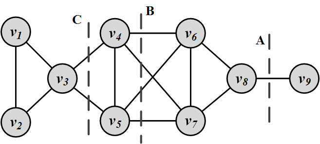
Edge-Betweennessis defined as the number of node pairs (v_i,v_j) such that the shortest path between v_i and v_j passes through e. For instance, in Figure 6.9(a), edge betweenness for edge e(1, 2) is 6/2 + 1 = 4, as all the shortest paths from 2 to \{4, 5, 6, 7, 8, 9\} have to either pass e(1, 2) or e(2, 3), and e(1,2) is the shortest path between 1 and 2. Formally, their algorithm is as follows
Girvan-Newman
Algorithm:
Calculate edge-betweeness for all edges in the graph;
Remove the edge with the highest betweenness;
Recalculate betweenness for all edges affected by the edge removal; and
Repeat until all edges are removed.
Consider the graph depicted in Figure 6.9(a). For this graph, the edge betweenness values are as follows:
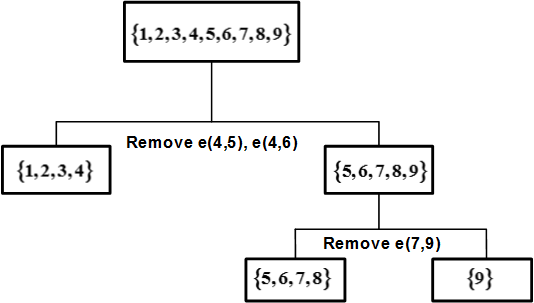
Therefore, by following the algorithm, the first edge that needs to be removed is e(4,5). By removing e(4,5), we compute the edge betweenness once again; this time, e(4,6) has the highest betweenness value: 20. This is because all shortest paths between nodes {1,2,3,4} to nodes {5,6,7,8,9} must pass e(4,6); therefore, it has betweenness 4\times 5=20. By following the steps of the algorithm, the dendrogram shown in Figure 6.9(b) can be obtained.
We discussed various community detection algorithms in this section. Figure 6.10 summarizes the two categories of community detection algorithms.
6.2 Community Evolution
So far we assume that networks are static. That is, nodes and edges are fixed and do not change over time. In reality, with the rapid growth of social media, networks and their internal communities change over time. Community detection algorithms need to be extended to deal with evolving networks. Before analyzing evolving networks, we need to answer the question, “How do networks evolve?" In this section, we discuss how networks evolve in general and then how communities evolve over time. We will demonstrate how communities can be found in these evolving networks.
6.2.1 How Networks Evolve
Large social networks are highly dynamic, where nodes and links appear or disappear over time.
In these evolving networks, many interesting patterns are observed. For instance, it is observed that when distances (in terms of shortest path distance) between two nodes increase, their probability of getting connected decreases2. We discuss three common patterns that are observed in evolving networks: segmentation, densification, and diameter shrinkage.
Network Segmentation
Often, in evolving networks, segmentation takes place, where the large network is decomposed over time into three parts:
Giant Component: As network connections stabilize, a giant component of nodes is formed with a large proportion of network nodes and edges falling into this component.
Stars: These are isolated parts of the network that form star structures. A star is a tree with one internal node and n leaves.
Singletons: These are orphan nodes disconnected from all nodes in the network.
Figure 6.11 depicts a segmented network and these three components.
Graph Densification
It is observed in evolving graphs that the density of the graph increases as the network grows. In other words, the number of edges increases faster than the number of nodes. This phenomenon is called densification. Let V(t) denote nodes at time t and let E(t) denote edges at time t,
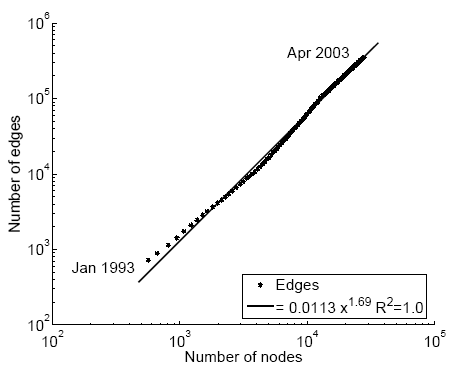
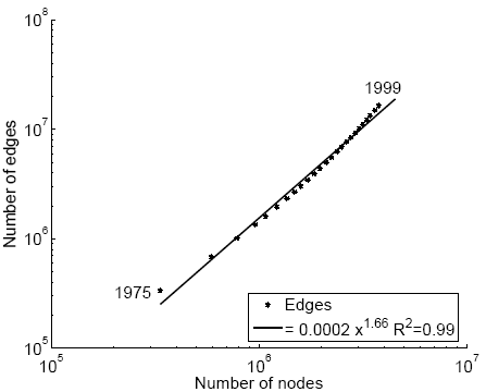
If densification happens, then we have 1 \le \alpha \le 2. There is linear growth when \alpha =1 and we get clique structures when \alpha=2 (why?). Networks exhibit \alpha values between 1 and 2 when evolving. Figure 6.12 depicts a log-log graph for densification for a physics citation network and a patent citation network. During the evolution process in both networks, the number of edges is recorded as the number of nodes grows. These recordings show that both networks have \alpha \approx 1.6, i.e., the log-log graph of |E| with respect to |V| is a straight line with slope 1.6. This value also implies that when V is given, in order to realistically model a social network, we should generate O(|V|^{1.6}) edges.
Diameter Shrinkage
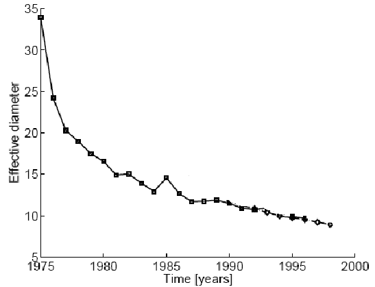
Another property observed in large networks is that the network diameter shrinks in time. This property has been observed in random graphs as well (see Chapter 4). Figure 6.13 depicts the diameter shrinkage for the same patent network discussed in Figure 6.12.
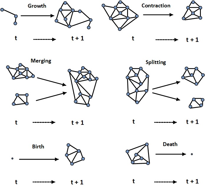
We discuss three phenomena that are observed in evolving networks. Communities in evolving networks also evolve. They appear, grow, shrink, split, merge, or even dissolve over time. Figure 6.14 depicts different situations that can happen during community evolution.
Both networks and their internal communities evolve over time. Given evolution information (e.g., when edges or nodes are added), how can we study evolving communities? And can we adapt static (non-temporal) methods to utilize this temporal information? We will discuss these next.
6.2.2 Community Detection in Evolving Networks
Consider an instant messaging (IM) application in social media. In these IM systems, members become “available" or “offline" frequently. Consider individuals as nodes and messages between them as edges. In this example, we are interested in finding a community of individuals that send messages to one another frequently. Clearly, community detection at any time stamp is not a valid solution since interactions are limited. A valid solution to this problem needs to utilize temporal information and interactions between users over time. We present community detection algorithms that incorporate temporal information. To incorporate temporal information, we can extend previously discussed static methods as follows:
Take t snapshots of the network, G_1, G_2, …, G_t, where G_i is a snapshot at time i;
Perform a static community detection algorithm on all snapshots independently; and
Assign community members based on communities found in all t different timestamps. For instance, we can assign nodes to communities based on voting. In voting, we assign nodes to communities they belong the most over time.
Unfortunately, this method is unstable in highly dynamic networks since community memberships are always changing. An alternative is to use evolutionary clustering.
Evolutionary Clustering
In evolutionary clustering, it is assumed that communities do not change most of the time; hence, it tries to minimize an objective function that considers both communities at different time stamps (snapshot cost or SC) and how they evolve throughout time (temporal cost or TC). Then, the objective function for evolutionary clustering is defined as a linear combination of snapshot cost and temporal cost (SC and TC) ,
where 0 \le \alpha \le 1. Let us assume spectral clustering (discussed in Section 1.1.3.1) is used to find communities at each timestamp. We know that the objective for spectral clustering is Tr(X^TLX) s.t. X^TX=I_m, so we will have the objective function at time t as
where X_t is the community membership matrix at time t. To define TC, we can compute the distance between the community assignments of two snapshots,
Unfortunately, this requires both X_t and X_{t-1} to have the same number of columns (number of communities). Moreover, X_t is not unique and can change by orthogonal transformations3; therefore, the distance value ||X_t-X_{t-1}||^2 can change arbitrarily. To remove the effect of orthogonal transformations and allow different numbers of columns, TC is defined as
where \frac{1}{2} is for mathematical convenience, and Tr(AB)=Tr(BA) is used. Therefore, evolutionary clustering objective can be stated as
Assuming normalized laplacian is used in spectral clustering, L=I-D_t^{-1/2}A_tD_t^{-1/2},
where \hat{L}=I - \alpha D_t^{-1/2}A_tD_t^{-1/2}-(1-\alpha)X_{t-1}X_{t-1}^T. Similar to spectral clustering, X_t can be obtained by taking the top eigenvectors of \hat{L}.
Note that at time t, we can obtain X_t directly by solving spectral clustering for the laplacian of the graph at time t, but then we are not employing any temporal information. Using evolutionary clustering and the new laplacian \hat{L}, we incorporate temporal information into our community detection algorithm and disallow user memberships in communities at time t: X_t to change dramatically from X_{t-1}.
6.3 Community Evaluation
When communities are found, one must evaluate how accurately the task has been performed. In terms of evaluating communities, the task is similar to evaluating clustering methods in data mining. Evaluating clustering is a challenge since ground truth may not be available. We will consider two scenarios: when ground truth is available, and when it is not.
6.3.1 Evaluation with Ground Truth
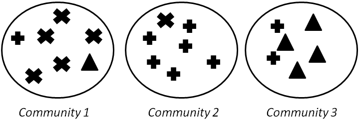
When ground truth is available, we have at least partial knowledge of what communities should look like. Here, we assume that we are given the correct community (clustering) assignments. We discuss 4 measures: Precision and Recall, F-Measure, Purity, and Normalized Mutual Information (NMI). Consider Figure 6.15, where 3 communities are found and the points are shown using their true labels.
Precision and Recall
Community detection can be considered a problem of assigning all similar nodes to the same community. In the simplest case, any two similar nodes should be considered members of the same community. Based on our assignments, four cases can occur:
True Positive (TP) Assignment: when similar members are assigned to the same community. This is a correct decision.
True Negative (TN) Assignment: when dissimilar members are assigned to different communities. This is a correct decision
False Negative (FN) Assignment: when similar members are assigned to different communities. This is an incorrect decision
False Positive (FP) Assignment: when dissimilar members are assigned to the same community. This is an incorrect decision
Precision (P) and Recall (R) are defined as follows,
Precision defines the fraction of pairs that have been correctly assigned to the same community. Recall discusses the fraction of pairs that the community detection algorithm assigned to the same community among the pairs that should have been in the same community.
We compute these values for Figure 6.15. For TP, we need to compute the number of pairs with the same label that are in the same community. For instance, for label \times and community 1, we have {5 \choose 2} such pairs. Therefore,
For FP, we need to compute dissimilar pairs that are in the same community. For instance, for community 1, this is (5 \times 1 + 5 \times 1 + 1 \times 1). Therefore,
FN computes similar members that are in different communities. For instance, for label +, this is (6 \times 1 + 6 \times 2 + 2 \times 1). Similarly,
Finally, TN computes the number of dissimilar pairs in dissimilar communities,
Hence,
F-Measure
To consolidate precision and recall into one measure, we can use the harmonic mean of precision and recall.
Computed for the same example, we get F=0.54.
Purity
In purity, we assume the majority of a community represents the community. Hence, we use the label of the majority against the label of each member to evaluate the algorithm. For instance, in Figure 6.15, and the majority in community 1 is \times; therefore, we assume majority label \times for that community. The purity is then defined as the fraction of instances that have labels equal to the community’s majority label. Formally,
where k is the number of communities, N is the total number of nodes, L_j is the set instances with label j in all communities, and M_i is the set of members in community i with the majority label. In the case of our example, purity is \frac{6+5+4}{20}=0.75.
Normalized Mutual Information
Purity can be easily tampered to generate high values; consider when nodes represent singleton communities (of size 1) or when we have very large pure communities (ground truth=majority label). In both cases, purity does not make sense since it generates high values.
A more precise measure to solve this problem is the Normalized Mutual Information (NMI), which originates in Information Theory. Mutual Information (MI) describes the amount of information two random variables share. In other words, by knowing one of the variables, NMI measures the amount of uncertainty reduced regarding the other variable. Consider the case of two independent variables; in this case, the mutual information is zero since knowing one does not help in knowing more information about the other. Mutual information of two variables X and Y is denoted as I(X,Y). We can use mutual information to measure the information one clustering carries regarding the ground truth. Mutual information can be calculated using Equation 6.56, where l and h are labels and found communities, n_{h} and n_{l} are the number of data points in the communities h and l respectively, n_{h,l} is the number of nodes in community h and label l, and n is the number of nodes.
Unfortunately, mutual information is unbounded; however, it is common for measures to have values in range [0,1]. To address this issue, we can normalize mutual information. We provide the following equation, without proof, which will help us normalize mutual information,
where H is the entropy function,
From Equation 6.57, we have MI \le H(L) and MI \le H(H); therefore,
Equivalently,
Equation 6.61 can be utilized to normalize mutual information. Thus, we introduce the Normalized Mutual Information (NMI) as
By plugging Equations 6.59, 6.58, and 6.56 into 6.62,
An NMI value close to one indicates high similarity between communities found and labels. A value close to zero indicates a long distance between them.
6.3.2 Evaluation without Ground Truth
When no ground truth is available, we can incorporate techniques based on semantics or clustering quality measures to evaluate community detection algorithms.
Evaluation with Semantics
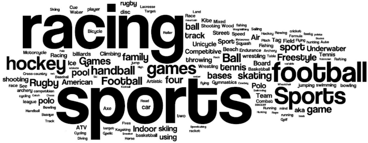
A simple way of analyzing detected communities is to analyze other attributes (posts, profile information, content generated, etc.) of community members in order to see if there is a coherency among community members. The coherency is often checked via human subjects. Amazon Mechanical Turk platform4 allows defining this task on its platform for human workers and hiring individuals from all around the globe to perform tasks such as community evaluation. To help analyze these communities, one can use word frequencies. By generating a list of frequent keywords for each community, human subjects determine whether these keywords represent a coherent topic. A more focused and single-topic set of keywords represents a coherent community. Tag clouds are one way of demonstrating these topics. Figure 6.16 depicts two coherent tag clouds for a community related to the US constitution and another for sports. Larger words in these tag clouds represent higher frequency of use.

Evaluation using Clustering Quality Measures
When experts are not available, an alternative is to use clustering quality measures. This approach is commonly employed when two or more community detection algorithms are available. Each algorithm is run on the target network and the quality measure is computed for the identified communities. The algorithm with a better quality measure value is considered a better algorithm. SSE (sum of squared errors), inter-cluster distance, among others can be used as a quality measure.
We can also follow this approach for evaluating a single community detection algorithm; however, we must ensure that the clustering quality measure used to evaluate community detection is different from the measure that was used to find communities. For instance, when using node similarity to group individuals, a measure other than node similarity should be used to evaluate the effectiveness of clustering.
6.4 Summary
In this chapter, we discuss communitiy analysis in social media. In particular, we answer three general questions: 1) how can we detection communities?, 2) How de communities evolve and how can we study evolving communities?, and 3) How can we evaluate detected communities? We start with a description of communities and how they are formed. Communities in social media are either explicit (emic) or implicit (etic). Community detection finds implicit communities in social media.
We review member-based and group-based community detection algorithms. In member-based community detection, we demonstrate how members can be grouped based on their degree, reachability, and similarity. For example, when using degrees, cliques are often considered as communities. Brute-force clique identification is employed to identify cliques. In practice, due to computational complexity of clique identifications, cliques are either relaxed or used as seeds of communities. We discuss k-plex as an example of relaxed cliques and clique percolation algorithm as an example of methods that use cliques as community seeds. When performing member-based community detection based on reachability, three frequently used subgraphs are k-clique, k-club, and k-clan. Finally, in member-based community detection based on node similarity, we discuss methods such as Jaccard and Cosine similarity that help compute node similarity. In group-based community detection, we show methods that find balanced, robust, modular, dense, or hierarchical communities. When finding balanced communities, one can employ spectral clustering. Spectral clustering provides a relaxed solution to normalized cut and ratio cuts in graphs. For finding robust communities, we search for subgraphs that are hard to disconnect. k-edge and k-vertex graphs are two examples of these robust subgraphs. For modular communities, we discuss modularity maximization, and for dense communities, we discuss quasi-cliques. Finally, hierarchical clustering is provided as a solution to finding hierarchical communities. Girvan-Newman algorithm is provided as an example.
In community evolution, we discuss when networks and, on a lower level, communities evolve. Furthermore, we discuss how commmunities can be detected in evolving networks using evolutionary clustering. Finally, we discuss how communities are evaluated when ground truth exists and when it does not.
6.5 Bibliographic Notes
A general survey of community detection in social media can be found in (Fortunato 2010) and a review of heterogeneous community detection in (Tang and Liu 2010). In related fields, (Berkhin 2006; Xu et al. 2005; Jain et al. 1999) provide surveys of clustering algorithms and (Faust and Wasserman 1994) provides a sociological perspective. Comparative analysis of community detection algorithms can be found in (Lancichinetti and Fortunato 2009) and (Leskovec et al. 2010). The description of explicit communities in this chapter is due to Kadushin (Kadushin 2012).
For member-based algorithm based on node degree, refer to (Kumar et al. 1999), which provides a systematic approach to finding clique-based communities with pruning. In algorithms based on node reachability, one can find communities by finding connected components in the network. For more information on finding connected components of a graph refer to (Hopcroft and Tarjan 1973). In node similarity, we discuss structural equivalence, similarity measures, and regular equivalence. More information on structural equivalence can be found in (Lorrain and White 1971; Leicht et al. 2006), on Jaccard similarity in (Jaccard 1901), and on regular equivalence in (Borgatti Martin and Stephen 1993).
In group-based methods that find balanced communities, we are often interested in solving the max-flow min-cut theorem. Linear programming (Cormen 2001), Ford-Fulkerson (Cormen 2001), Edmonds-Karp (Edmonds and Karp 1972), and Push-Relabel (Goldberg and Tarjan 1988) methods are some established techniques for solving the max-flow min-cut problem. We discuss quasi-cliques that help find dense communities. Finding the maximum quasi-clique is discussed in (Pattillo et al. 2012). A well known greedy algorithm for finding quasi-cliques is introduced by (Abello et al. 2002). In their approach a local search with a pruning strategy is performed on the graph to enhance the speed of quasi-clique detection. In their pruning strategy, a peel strategy is defined, where vertices that have some degree k along with their incident edges are recursively removed. There is a variety of algorithms to find dense subgraphs such as the one discussed in (Gibson et al. 2005) where the authors propose an algorithm that recursively fingerprints the graph (shindling algorithm) and creates dense-subgraphs. In group-based methods that find hierarchical communities, we detail hierarchical clustering. Hierarchical clustering algorithms are usually variants of single link, average link or complete link algorithms (Jain and Dubes 1988). In hierarchical clustering, COBWEB (Fisher 1987) and CHAMELEON (Karypis et al. 1999) can be named as two well known algorithms. In group-based community detection, Latent space models (Handcock et al. 2007; Hoff et al. 2002) are also very popular, which is not discussed in this chapter. In addition to the topics discussed in this chapter, community detection can also be performed for networks with multiple types of interaction (edges) (Tang and Liu 2009; Tang et al. 2012). We also restricted our discussion to community detection algorithms that use graph information. One can also perform community detection based on the content individuals share on social media. For instance, utilizing tagging relation (i.e., individuals that shared the same tag) (Wang et al. 2010), instead of connections between users, one can discover overlapping communities, which provides a natural summarization to the interests of the identified communities.
In network evolution analysis, network segmentation is discussed in (Kumar et al. 2010). Segment-based clustering (Sun et al. 2007) is another method not covered in this chapter.
NMI was first introduced in (Strehl et al. 2003) and in terms of clustering quality measures, Davies-Bouldin (Davies and Bouldin 1979) measure, Rand index (Rand 1971), C-index (Dunn 1974), Silhouette index (Rousseeuw 1987), and Goodman-Kruskal index (Goodman and Kruskal, n.d.) can be used.
6.6 Exercises
Provide an example to illustrate how community detection can be subjective.
Community Detection
Given a complete graph K_n, how many nodes will the Clique Percolation Method generate for the clique graph for value k? How many edges will it generate?
Find all k-cliques, k-clubs, and k-clans in a complete graph of size 4.
For a complete graph of size n, is it m-connected? What possible values can m take?
Why is the smallest eigenvector meaningless when using an unnormalized laplacian matrix?
Modularity can be defined as
Q = \frac{1}{2m} \sum_{ij} \left[ A_{ij} - \frac{k_i k_j}{2m} \right] \delta(c_i,c_j),(6.64)where \delta(c_i,c_j) (Kronecker delta) is 1 when c_i and c_j both belong to the same community and 0 otherwise.
What is the range [\alpha_1, \alpha_2] for Q values? Provide examples for both extreme values of the range as well as cases where modularity becomes zero.
What are the limitations for modularity? Provide an example where modularity maximization does not seem reasonable.
Find 3 communities in Graph 6.8 by performing modularity maximization.
For graph 6.8:
Compute Jaccard and Cosine similarity between nodes 4 and 8, assuming the neighborhood of a node excludes the node itself.
Compute Jaccard and Cosine similarity when the node is included in the neighborhood
Community Evolution
What is the upper bound on densification factor \alpha? Explain.
Community Evaluation
Normalized Mutual Information (NMI) is used to evaluate clustering results when the actual clustering of the data (the number of clusters and the clustering assignments) is known beforehand.
What are the maximum and minimum values for the NMI? Provide details.
Explain how NMI works (describe the intuition behind it).
Compute NMI for Figure 6.15.
Why is high precision not enough? Provide an example to show that both precision and recall are important.
Discuss situations where purity does not make sense.
Compute the following for Figure 6.17:
Figure 6.17: Commmunity Evaluation Example Precision and Recall
F-Measure
NMI
Purity
For more details refer to (Chung 1997).↩︎
See (Kossinets and Watts 2006) for details.↩︎
Let X be the solution to spectral clustering. Consider an orthogonal matrix Q, i.e., QQ^T=I. Let Y=XQ. In spectral clustering, we are maximizing Tr(X^TLX)=Tr(X^TLXQQ^T)=Tr(Q^TX^TLXQ)=Tr((XQ)^TL(XQ))=Tr(Y^TLY). In other words, Y is another answer to our trace maximization problem. This proves that the solution X to spectral clustering is non-unique under orthogonal transformations Q.↩︎
http://www.mturk.com↩︎