Network Models
In May 2011, Facebook had 721 million users, represented by a graph of 721 million nodes. A Facebook user at the time had an average of 190 friends, that is, all Facebook users taken into account, a total of 68.5 billion friendships, i.e., edges. What are the principal underlying processes that help initiate these friendships? More importantly, how can these seemingly independent friendships form this complex friendship network?
In social media, many social networks contain millions of nodes and billions of edges. To understand these complex networks, we are faced with billions of friendships, the reasons for the existence of most of which are obscure. Humbled by the complexity of these networks and the difficulty to independently analyze each one of these friendships, we design models that generate, on a smaller scale, graphs similar to real-world networks. Hoping that these models simulate properties observed in real-world networks well, the analysis of real-world networks boils down to a cost-efficient measuring of different properties of simulated networks. In addition, these models
Allow for a better understanding of phenomena observed in real-world networks by providing concrete mathematical explanations; and
Allow for controlled experiments on synthetic networks when real-world networks are not available.
We discuss three principal network models in this chapter: the random graph model, the small-world model, and the preferential attachment model, designed to accurately model properties observed in real-world networks. Before we delve into the details of these models, we discuss these properties of real-world networks.
4.1 Properties of Real-World Networks
Real-world networks share common characteristics. When designing network models, we aim to devise models that can accurately describe these networks by mimicking these common characteristics. To determine characteristics shared by real-world networks, a regular practice is to utilize their attributes and show that measurements for these attributes are consistent across networks. In particular, three network attributes exhibit consistent measurements across real-world networks: degree distribution, clustering coefficient, and average path length. Degree distribution denotes how node degrees are distributed across a network. Clustering coefficient measures transitivity in a network. Finally, average path length denotes the average distance (shortest path length) between pairs of nodes. We discuss how these three attributes behave in real-world networks next.
4.1.1 Degree Distribution
Consider the distribution of wealth among individuals. Most individuals have average capitals, whereas a few are considered wealthy. In fact, we observe exponentially more individuals with average capital than the wealthier ones. Similarly, consider the population of cities. Often, a few metropolitan areas are densely populated, whereas other cities have an average population size. In social media, we observe the same phenomenon regularly when measuring popularity or interestingness for entities. For instance,
Many sites are visited less than a 1,000 times a month whereas a few are visited more than a million times daily.
Social media users are often active on a few sites whereas some individuals are active on hundreds of sites.
There are exponentially more modestly priced products for sale compared to expensive ones.
There exist many individuals with a few friends and a handful of users with thousands of friends.
The last observation is directly related to node degrees in social media. Degree of a node in social media often denotes the number of friends an individual has. Thus, the distribution of number of friends denotes the degree distribution of the network. It turns out that in all provided examples, the distribution of values follows power-law distribution
Power-Law
Distribution. For instance, let k denote the degree of a node, i.e., the number of friends an individual has. Let f(k) denote the number of individuals with degree k, i.e., frequency of observing k. Then, in power-law distribution
where b is the power-law exponent and a is the power-law intercept. A power-law degree distribution is shown in Figure 4.1(a).
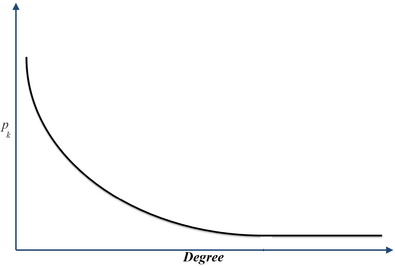
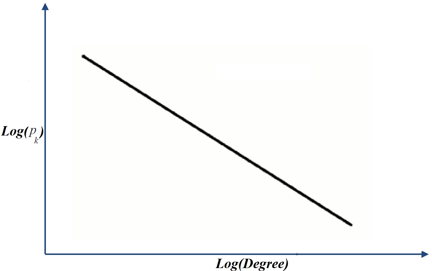
Taking the logarithm from both sides of Equation 4.1, we get
This equation shows that the log-log plot of a power-law distribution is a straight line with slope -b and intercept \ln a (see Figure 4.1(b)). This also reveals a methodology for checking whether a network exhibits power-law distribution. We can
Pick a popularity measure and compute it for the whole network. For instance, we can take the number of friends in a social network as a measure. We denote the measured value as k.
Compute f(k), the number of individuals having popularity k.
Plot a log-log graph, where the x-axis represents \ln k and the y-axis represents \ln f(k).
If a power-law distribution exists, we should observe a straight line in the plot.
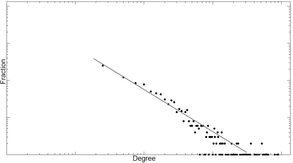
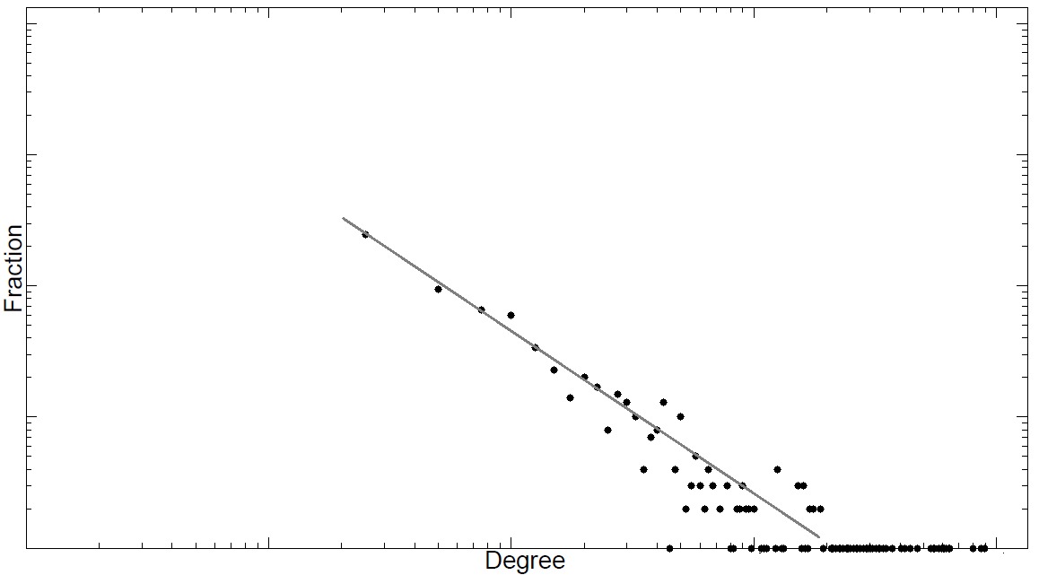
Figure 4.2 depicts some log-log graphs for the number of friends on real-world networks. In all networks, a linear trend is observed denoting a power-law degree distribution.
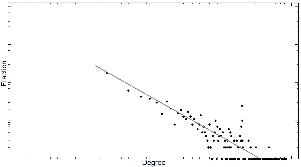
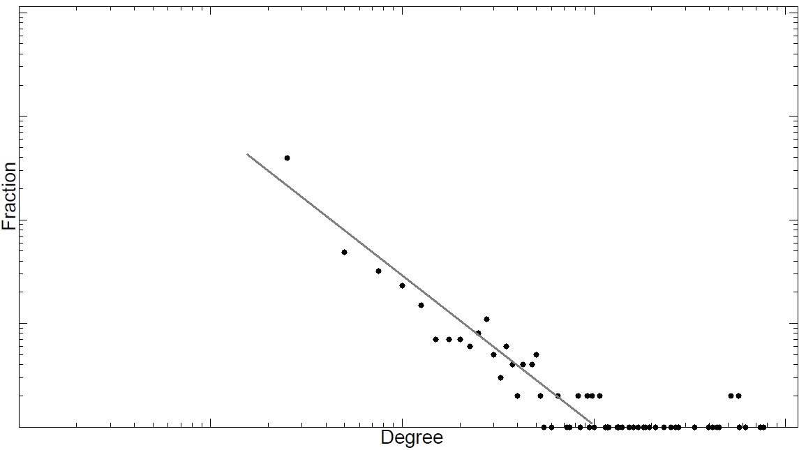
Networks exhibiting power-law degree distribution are often called scale-free
Scale-free
Networksnetworks. Since the majority of social networks are scale-free, we are interested in models that can generate synthetic networks with power-law degree distribution.
4.1.2 Clustering Coefficient
In real-world social networks, friendships are highly transitive. In other words, friends of an individual are often friends with one another. These friendships form triads of friendships that are frequently observed in social networks. These triads result in networks with high average [local] clustering coefficients. In May 2011, Facebook had an average clustering coefficient of 0.5 for individuals who had two friends, i.e., their degree was 2 (Ugander et al., n.d.). This indicates that for 50% of all users with 2 friends, their two friends were also friends with each other. Table 1.1 provides the average clustering coefficient for real-world social network and the web.
| Web | Flickr | LiveJournal | Orkut | YouTube | |
|---|---|---|---|---|---|
| 0.081 | 0.14 (with 100 friends) | 0.31 | 0.33 | 0.17 | 0.13 |
4.1.3 Average Path Length
In real-world networks, any two members of the network are usually connected via short paths. In other words, the average path length is small. This is known as the small-world phenomenon
Small-world and
Six Degrees of
Separation. In the well-known small-world experiment conducted in the 1960’s by Stanley Milgram, Milgram conjectured that people around the world are connected to one another via a path of at most 6 individuals, i.e., the six degrees of separation. Similarly, we observe small average path lengths in social networks. For example, in May 2011, the average path length between individuals in the Facebook graph was 4.7. This average was 4.3 for individuals in the US at the same time (Ugander et al., n.d.). Table 1.2 provides the average path length for real-world social network and the web.
| Web | Flickr | LiveJournal | Orkut | YouTube | |
|---|---|---|---|---|---|
| 16.12 | 4.7 | 5.67 | 5.88 | 4.25 | 5.10 |
The above three properties are consistently observed in real-world networks. We design models based on simple assumptions on how friendships are formed, hoping that these models generate scale-free networks, with high clustering coefficient and small average path lengths. We start with the simplest network model, the random graph model, next.
4.2 Random Graphs
We start with the most basic assumption on how friendships can be formed. That is,
Edges (i.e., friendships) between nodes (i.e., individuals) are formed randomly.
The random graph model follows this basic assumption. In reality friendships in real-world networks are far from random. By assuming random friendships, we simplify the process of friendship formation in real-world networks, hoping that these random friendships ultimately create networks that exhibit common characteristics observed in real-world networks.
Formally, we can assume that for a graph with a fixed number of nodes n, any of the {n \choose 2} edges can be formed independently, with probability p. This graph is called a random graph and we denote it as G(n,p) model.
G(n,p). This model was first proposed independently by Edgar Gilbert (Gilbert 1959) and Solomonoff and Rapoport (Solomonoff and Rapoport 1951). Another way of randomly generating graphs is to assume both number of nodes n and number of edges m are fixed. However, we need to determine which m edges are selected from the set of {n \choose 2} possible edges. Let \Omega denote the set of graphs with n nodes and m edges. To generate a random graph, we can uniformly select one of the graphs in \Omega. The number of graphs with n nodes and m edges, i.e., |\Omega|, is
The uniform random graph selection probability is \frac{1}{|\Omega|}. One can think of the probability of uniformly selecting a graph as an analog to p, the probability of selecting an edge in G(n,p).
The second model was introduced by Paul Erdős and Alfred Rényi (Erdős and Rényi 1959) and is denoted as G(n,m) model
G(n,m). In the limit, both models act similarly. The expected number of edges in G(n,p) is {n \choose 2}p. Now, if we set {n \choose 2}p=m in the limit, both models act the same since they contain the same number of edges. Note that the G(n,m) model contains a fixed number of edges; however, the second model G(n,p) is likely to contain none or all possible edges.
Mathematically, the G(n,p) model is almost always simpler to analyze; hence the rest of this section deals with properties of this model. Note that there exist many graphs with n nodes and m edges, i.e., generated by G(n,m). The same argument holds for G(n,p) and many graphs can be generated by the model. Therefore, when measuring properties in random graphs, the measures are calculated over all graphs that can be generated by the model and then averaged. This is particularly useful when we are interested in the average, and not specific, behavior of large graphs.
In G(n,p), the number of edges are not fixed; therefore, we first examine some mathematical properties regarding the expected number of edges that are connected to a node, the expected number of edges observed in the graph, and the likelihood of observing m edges in a random graph generated by the G(n,p) process.
The expected number of edges connected to a node (expected degree) in G(n,p) is (n-1)p.
Proof. A node can be connected to at most n-1 nodes (via n-1 edges). All edges are selected independently with probability p. Therefore, on average (n-1)p of them are selected. The expected degree is often denoted using notation c or k in the literature. Since we frequently use k to denote degree values, we use c to denote the expected degree of a random graph,
or equivalently,
The expected number of edges in G(n,p) is {n \choose 2}p.
Proof. Following the same line of argument, since edges are selected independently and we have a maximum of {n \choose 2} edges, the expected number of edges is {n \choose 2}p. ◻
In a graph generated by G(n,p) model, the probability of observing m edges is
Proof. m edges are selected from the {n \choose 2} possible edges. These edges are formed with probability p^m and other edges are not formed (to guarantee the existence of only m edges) with probability (1-p)^{{n \choose 2}-m}. ◻
Given these basic propositions, we next analyze how random graphs evolve as we add edges to them.
4.2.1 Evolution of Random Graphs
In random graphs, when nodes form connections, after some time, a large fraction of nodes get connected, i.e., there is a path between any pair of them. This large fraction forms a connected component, commonly called the largest connected component
Giant Componentor the giant component. We can tune the behavior of the random graph model by selecting the appropriate p value. In G(n,p), when p=0, the size of the largest connected component is 0 (no two pairs are connected) and, when p=1, the size is n (all pairs are connected). Table 1.3 provides the size of the largest connected component (slc in the Figure) for random graphs with 10 nodes and different p values. The figure also provides information on the average degree c, the diameter size ds, the size of the largest component slc, and the average path length l of the random graph.
 |
 |
 |
 |
|
|---|---|---|---|---|
| p | 0.0 | 0.055 | 0.11 | 1.0 |
| c | 0.0 | 0.8 | \approx 1 | 9.0 |
| ds | 0 | 2 | 6 | 1 |
| slc | 0 | 4 | 7 | 10 |
| l | 0.0 | 1.5 | 2.66 | 1.0 |
As shown, in Table 1.3, as p gets larger, the graph gets denser. When p is very small,
No giant component is observed in the graph;
Small isolated connected components are formed; and
The diameter is small since all nodes are in isolated components, in which they are connected to a handful of other nodes.
As p gets larger,
A giant component starts to appear;
Isolated components become connected; and
The diameter values get larger.
At this point, nodes are connected to each other via long paths (see p=0.11 in Table 1.3). As p continues to get larger, the random graph properties change again. For larger values, the diameter starts shrinking since nodes get connected to each other via different paths (that are likely to be shorter). The point where diameter value starts to shrink in a random graph is called Phase Transition
Phase Transition. At the point of Phase Transition, the following phenomena are observed,
The giant component that just started to appear, starts to grow, and
The diameter that just reached its maximum value, starts decreasing.
It is proven that in random graphs, phase transition occurs when c=1, i.e., p=1/(n-1).
In random graphs, phase transition happens at c=1.
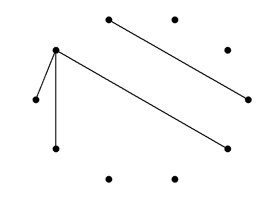
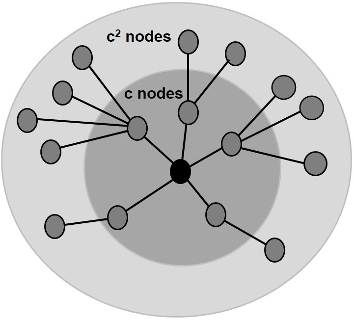
Proof. (Sketch) Consider a random graph with expected node degree c, where c=p(n-1). In this graph, consider any connected set of nodes S and consider the complement set \bar{S}=V-S. For the sake of our proof, we assume that |S|<<\bar{S}. Given any node v in S, if we move one hop (edge) away from v, we visit approximately c nodes. Following the same argument, if we move one hop away from nodes in S, we visit approximately |S|c nodes. Assuming |S| is small, the nodes in S only visit nodes in \bar{S} and when moving one hop away from S, the set of nodes “guaranteed to be connected" gets larger by a factor c (see Figure 4.3). The connected set of visited nodes gets c^2 times larger when moving 2 hops and so on. Now, in the limit, if we want this component of visited nodes to become the largest connected component, then after traveling n hops, we must have
Otherwise, i.e., c < 1, the number of visited nodes dies out exponentially. Hence, phase transition happens at c=1 1. ◻
Note that this proof sketch provides an intuitive approach to understand the proposition. Interested readers can refer to bibliographic notes for a concrete proof.
We have discussed generation and evolution of random graphs; however, we also need to analyze how random graphs perform in terms of mimicking properties exhibited by real-world networks. It turns out that random graphs can model average path length in a real-world network accurately, but fail to generate a realistic degree distribution or clustering coefficient. We discuss these properties next.
4.2.2 Properties of Random Graphs
Degree Distribution
When computing degree distribution, we estimate the probability of observing P(d_v=d) for node v.
For a graph generated by G(n,p), node v has degree d, d \le n-1, with probability
Proof. Left to the reader 2. ◻
This assumes that n is fixed. We can generalize this result by computing degree distribution of random graphs in the limit, i.e., n \rightarrow \infty. In this case, using Equation 4.4 and the fact that \lim_{x \rightarrow 0} \ln (1+x) = x, we can compute the limit for each term of Equation 4.8,
We also have
We can compute the degree distribution of random graphs in the limit by substituting Equations 4.14, 4.10, and 4.4 in Equation 4.8,
which is basically the Poisson distribution with mean c. Thus, in the limit, random graphs generate Poisson degree distributions, which is different from the power-law degree distribution observed in real-world networks.
Clustering Coefficient
In a random graph generated by G(n,p), the expected local clustering coefficient for node v is p.
Proof. The local clustering coefficient for node v is
However, v can have different degrees depending on the edges that are formed randomly. Thus, we can compute the expected value for C(v),
The first term is basically the clustering coefficient of a node given its degree. For a random graph, we have
Substituting Equation 4.19 in Equation 4.17, we get
where we have used the fact that all probability distributions sum up to 1. ◻
The global clustering coefficient of a random graph generated by G(n,p) is p.
Proof. The global clustering coefficient of a graph defines the probability of two neighbors of the same node being connected. In random graphs, for any two nodes, this probability is the same and is equal to the generation probability p that determines the probability of two nodes getting connected. Note that in random graphs, the expected local clustering coefficient is equivalent to the global clustering coefficient. ◻
In random graphs, the clustering coefficient is equal to the probability p; therefore, by appropriately selecting p, we can generate networks with high clustering coefficient. Note that selecting a large p is undesirable as it will generate a very dense graph, which is unrealistic, as in the real-world, networks are often sparse. Thus, random graphs are considered generally incapable of generating networks with high clustering coefficients without compromising other required properties.
Average Path Length
The average path length in a random graph is
Proof. (Sketch) The proof is similar to the proof provided in determining when phase transition happens (see Section 1.2.1). Let \mathcal{D} denote the expected diameter size in the random graph. Starting with any node in a random graph and its expected degree c, one can visit approximately c nodes by traveling one edge, c^2 nodes by traveling 2 edges, and c^{\mathcal{D}} nodes by traveling “diameter" number of edges. After this step, almost all nodes should be visited. In this case, we have
In random graphs, the expected diameter size tends to the average path length l in the limit. This we provide without proof. Interested readers can refer to bibliographic notes for pointers to concrete proofs. Using this fact, we have
Taking the logarithm from both sides we get l\approx \frac{\ln |V|}{\ln c}. Therefore, the average path length in a random graph is equal to \frac{\ln |V|}{\ln c}. ◻
4.2.3 Modeling Real-World Networks with Random Graphs
Given a real-world network, we can simulate it using a random graph model. We can compute the average degree c in the given network. From c, the connection probability p can be computed (p=\frac{c}{n-1}). Using p and the number of nodes in the given network n, random graph model G(n,p) can be simulated. Table 1.4 demonstrates the simulation results for various real-world networks. As observed in the table, random graphs perform well in modeling the average path lengths; however, when considering the transitivity, the random graph model drastically underestimates the clustering coefficient.
| Original Network | Simulated Random Graph | |||||
|---|---|---|---|---|---|---|
| Network | Size | Average Degree | Average Path Length | C | Average Path Length | C |
| Film Actors | 225,226 | 61 | 3.65 | 0.79 | 2.99 | 0.00027 |
| Medline Coauthorship | 1,520,251 | 18.1 | 4.6 | 0.56 | 4.91 | 1.8 \times 10^{-4} |
| E.Coli | 282 | 7.35 | 2.9 | 0.32 | 3.04 | 0.026 |
| C.Elegans | 282 | 14 | 2.65 | 0.28 | 2.25 | 0.05 |
To tackle this issue, we study the small-world model.
4.3 Small-World Model
The assumption behind the random graph model is that connections in real-world networks are formed at random. Although unrealistic, random graphs can model average path lengths in real-world networks properly, but underestimate the clustering coefficient. To mitigate this problem, Duncan J. Watts and Steven Strogatz in 1997 (Watts and Strogatz 1998) proposed the small-world model.
In real-world interactions, many individuals have a limited and often at least, a fixed number of connections. Individuals connect with their parents, brothers, sisters, grandparents, and teachers, among others. Thus, instead of assuming random connections, as we did in random graph models, one can assume an egalitarian model in real-world networks, where people have the same number of neighbors (friends). This again is unrealistic; however, it better models the clustering coefficient of real-world networks.
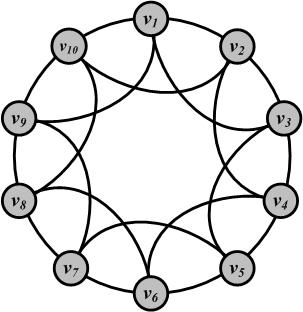
Regular Ring LatticeIn graph theory terms, this assumption is equivalent to embedding individuals in a regular network. A regular (ring) lattice is a special case of regular networks where there exists a certain pattern on how ordered nodes are connected to one another. In particular, in a regular lattice of degree c, nodes are connected to their previous c/2 and following c/2 neighbors. Formally, for node set V=\{v_1, v_2, v_3, \dots, v_n\}, an edge exists between node v_i and v_j if and only if
A regular lattice of degree 4 is shown in Figure 4.4.
The regular lattice can model transitivity well; however, the average path length is too high. Moreover, the clustering coefficient takes the value
which is fixed and not tunable to clustering coefficient values found in real-world networks. To overcome these problems, the proposed small-world model dynamically lies between the regular lattice and the random network.
In the small-world model, we assume a parameter \beta controls randomness in the model. The model starts with a regular lattice and starts adding random edges based on \beta. The 0 \le \beta \le 1 controls how random the model is. When \beta is 0, the model is basically a regular lattice, and when \beta=1, the model becomes a random graph.
The procedure for generating small-world networks is outlined in Algorithm 4.1. The procedure creates new edges by a process called rewiring. Rewiring will replace an existing edge between nodes v_i and v_j with a non-existing edge between v_i and v_k with probability \beta. In other words, an edge is disconnected from one of its endpoints v_j and connected to a new endpoint v_k. Node v_k is selected uniformly.
- Require: Number of nodes |V|, mean degree c, parameter \beta
- return A small-world graph G(V,E)
- G= A regular ring lattice with |V| nodes and degree c
- for node v_i (starting from v_1), and all edges e(v_i,v_j), i < j do
- v_k=Select a node from V uniformly at random.
- if rewiring e(v_i,v_j) to e(v_i,v_k) does not create loops in the graph or multiple edges between v_i and v_k then
- rewire e(v_i,v_j) with probability \beta: E=E-\{e(v_i,v_j)\}, E=E \cup \{e(v_i,v_k)\};
- end if
- end for
- Return G(V,E)
The network generated using this procedure has some interesting properties. Depending on the \beta value, it can have a high clustering coefficient and also short average path lengths. The degree distribution however still does not match that of real-world networks.
4.3.1 Properties of the Small-World Model
Degree Distribution
The degree distribution for the small-world model is as follows,
where P(d_v=d) is the probability of observing degree d for node v. We provide this equation without proof due to techniques beyond the scope of this book (see Bibliographic Notes). Note that the degree distribution is quite similar to the Poisson degree distribution observed in random graphs (Section 1.2.2). In practice, in the graph generated by the small-world model, most nodes have similar degrees due to the underlying lattice. In contrast, in real-world networks, degrees are distributed based on power-law distribution, where most nodes have small degrees and a few have large degrees.
Clustering Coefficient
The clustering coefficient for a regular lattice is \frac{3(c-2)}{4(c-1)}. The clustering coefficient for a random graph model is p=\frac{c}{n-1}. The clustering coefficient for a small-world network is a value between these two, depending on \beta. Commonly, the clustering coefficient for a regular lattice is represented using C(0) and the clustering coefficient for a small-world model with \beta=p is represented as C(p). The relation between the two values can be computed analytically; it has been proven that
The intuition behind this relation is that since clustering coefficient enumerates the number of closed triads in a graph, we are interested in triads that are still left connected after the rewiring process. For a triad to stay connected, all three edges must not be rewired with probability (1-p). Since the process is performed independently for each edge, the probability of observing triads is (1-p)^3 times the probability of observing them in a regular lattice. Note that we also need to take into account new triangles that are formed by the rewiring process; however, that probability is nominal and hence, negligible. The graph in Figure 4.5 depicts the value of \frac{C(p)}{C(0)} for different values of p.
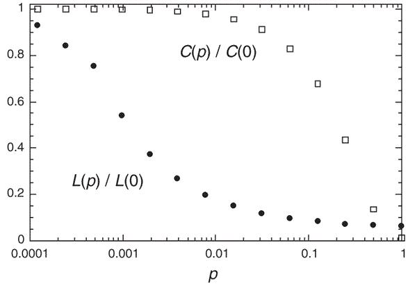
As shown in the figure, the value for C(p) stays high until p reaches 0.1 (10% rewired) and then decreases rapidly to a value around zero. Since high clustering coefficient is required in generated graphs, \beta \le 0.1 is preferred.
Average Path Length
The same procedure can be done for the average path length. The average path length in a regular lattice is
We denote this value as l(0). The average path length in a random graph is \frac{\ln n}{\ln k}. We denote l(p) as the average path length for a small-world model where \beta=p. Unlike C(p), no analytical formula for comparing l(p) to l(0) exists; however, the relation can be computed empirically for different values of p. Similar to C(p), we plot \frac{l(p)}{l(0)} in Figure 4.5. As shown in the figure, the average path length decays sooner than the clustering coefficient and becomes stable when around 1% of edges are rewired. Since we require small average path lengths in the generated graphs, \beta \ge 0.01 is preferred.
4.3.2 Modeling Real-World Networks withthe Small-World Model
A desirable model for a real-world network should generate graphs with high clustering coefficients and short average path lengths. As shown in Figure 4.5, for 0.01 \le \beta \le 0.10, the small-world network generated is acceptable, in which average path length is small and the clustering coefficient is still high. Given a real-world network in which average degree c and clustering coefficient C is given, we set C(p)=C and determine \beta using equation 4.27. Given \beta, c, and n (size of the real-world network), we can simulate the small-world model.
Table 1.5 demonstrates the simulation results for various real-world networks. As observed in the table, the small-world model generates realistic clustering coefficient and small average path length. Note that the small-world model is still incapable of generating a realistic degree distribution in the simulated graph. To generate scale-free networks (i.e., with power-law degree distribution), we introduce the preferential attachment model next.
| Original Network | Simulated Graph | |||||
|---|---|---|---|---|---|---|
| Network | Size | Average Degree | Average Path Length | C | Average Path Length | C |
| Film Actors | 225,226 | 61 | 3.65 | 0.79 | 4.2 | 0.73 |
| Medline Coauthorship | 1,520,251 | 18.1 | 4.6 | 0.56 | 5.1 | 0.52 |
| E.Coli | 282 | 7.35 | 2.9 | 0.32 | 4.46 | 0.31 |
| C.Elegans | 282 | 14 | 2.65 | 0.28 | 3.49 | 0.37 |
4.4 Preferential Attachment Model
There exist a variety of scale-free network modeling algorithms. A well-established one is the model proposed by Barábasi and Albert (Barabási and Albert 1999). The model is called preferential attachment or sometimes the Barábasi-Albert (BA) model, and is as follows:
When new nodes are added to networks, they are more likely to connect to existing nodes that many others have connected to.
This connection likelihood is proportional to the degree of the node that the new node is aiming to connect to. In other words, a rich-get-richer phenomenon or aristocrat network is observed where the higher the node’s degree, the higher the probability of new nodes getting connected to it. Unlike random graphs in which we assume friendships are formed randomly, in preferential attachment model we assume individuals are more likely to befriend gregarious others. The model’s algorithm is provided in Algorithm 4.2.
- Require: Graph G(V_0,E_0), where |V_0|=m_0 and d_v \ge 1 $
- for all do ~v\in V_0, number of expected connections m \le m_0, time to run the algorithm t$
- return A scale-free network
//Initial graph with m_0 nodes with degrees at least 1- G(V,E)= G(V_0,E_0);
- for 1 to t do
- V=V \cup \{v_i\};
// add new node v_i - while d_{i} \neq m do
- Connect v_i to a random node v_j \in V, i \neq j (~i.e., E=E\cup \{e(v_i,v_j)\}~)\\with probability P(v_j)=\frac{d_j}{\sum_k d_k}.
- end while
- end for
- Return G(V,E)
The algorithm starts with a graph containing a small set of nodes m_0, then adds new nodes one at a time. Each new node gets to connect to m \le m_0 other nodes and each connection to existing node v_i depends on the degree of v_i, i.e., P(v_i)=\frac{d_i}{\sum_j d_j}. Intrinsically, higher degree nodes get more attention from newly added nodes. Note that the initial m_0 nodes must have at least degree 1 for probability P(v_i)=\frac{d_i}{\sum_j d_j} to be non-zero.
The model incorporates two ingredients: 1) the growth element and 2) the preferential attachment element, to achieve a scale-free network. The growth is realized by adding nodes as time goes by. The preferential attachment is realized by connecting to node v_i based on its degree probability, P(v_i)=\frac{d_i}{\sum_j d_j}. Removing any one of these ingredients generates networks that are not scale-free (see Exercises). Next, we show that preferential attachment models are capable of generating networks with power-law degree distribution. Preferential attachment models are also capable of generating small average path length but unfortunately fail at generating the high clustering coefficients observed in real-world networks.
4.4.1 Properties of the Preferential Attachment Model
Degree Distribution
We first demonstrate that the preferential attachment model generates scale-free networks and can therefore model real-world networks. Empirical evidence found by simulating the preferential attachment model suggests that this model generates a scale free network with exponent b=2.9 \pm 0.1 (Barabási and Albert 1999). Theoretically, a mean-field (Newman and Watts 2006) proof can be provided as follows.
Let d_i denote the degree for node v_i. The probability of an edge connecting from a new node to v_i is
The expected increase to the degree of v_i is proportional to d_i (this is true on average). Assuming a mean-field setting, the expected temporal change in d_i is
Note that at each time step, m edges are added; therefore, mt edges are added over time and the degree sum \sum_j d_j is 2mt. Rearranging and solving this differential equation, we get
Here, t_i represents the time v_i was added to the network and since we set the expected degree to m in preferential attachment, then d_i(t_i)=m.
The probability that d_i is less than d is
Assuming uniform intervals of adding nodes,
The factor \frac{1}{(t+m_0)} shows the probability that one time step has passed since at the end of simulation, t+m_0 nodes are in the network. The probability density for P(d) is what we are interested in,
which, when solved, gives the stationary solution,
which is a power-law degree distribution with exponent b=3. Note that in real-world networks, the exponent varies in a range, e.g., [2,3]; however, there is no variance in the exponent of the introduced model. To overcome this issue, several other models are proposed. Interested readers can refer to bibliographical notes for further references.
Clustering Coefficient
In general, not many triangles are formed by the Barábasi-Albert model, since edges are created independently and one at a time. Again, using a mean-field analysis, the expected clustering coefficient can be calculated as
where t is the time passed in the system during the simulation. We avoid the details due to techniques beyond the scope of this book. Unfortunately, as time passes, the clustering coefficient gets smaller and fails to model the high clustering coefficient observed in real-world networks.
Average Path Length
The average path length of the preferential attachment model increases logarithmically with the number of nodes present in the network,
This indicates that, on average, preferential attachment models generate shorter path lengths than random graphs. Random graphs are considered accurate in approximating the average path lengths. The same holds for preferential attachment models.
4.4.2 Modeling Real-World Networks withthe Preferential Attachment Model
Similar to random graphs, we can simulate real-world networks by generating a preferential attachment model by setting the expected degree m (see Algorithm 4.2). Table 1.6 demonstrates the simulation results for various real-world networks. The preferential attachment model generates realistic degree distribution and as observed in the table, small average path lengths; however, the generated networks fail to exhibit the high clustering coefficient observed in real-world networks.
| Original Network | Simulated Graph | |||||
|---|---|---|---|---|---|---|
| Network | Size | Average Degree | Average Path Length | C | Average Path Length | C |
| Film Actors | 225,226 | 61 | 3.65 | 0.79 | 4.90 | \approx 0.005 |
| Medline Coauthorship | 1,520,251 | 18.1 | 4.6 | 0.56 | 5.36 | \approx 0.0002 |
| E.Coli | 282 | 7.35 | 2.9 | 0.32 | 2.37 | 0.03 |
| C.Elegans | 282 | 14 | 2.65 | 0.28 | 1.99 | 0.05 |
4.5 Summary
In this chapter, we discussed well-established models that generate networks with commonly observed characteristics is real-world networks. In particular, we explored random graphs, the small-world model, and preferential attachment. In random graphs, we assume connections are completely random. We discussed two variants of random graphs, G(n,p) and G(n,m). Random graphs exhibit a Poisson degree distribution, a small clustering coefficient p, and a realistic average path length \frac{\ln |V|}{\ln c}.
In the small-world model, we assume individuals have a fixed number of connections in addition to random connections. This model generates networks with high transitivity and short path lengths, both commonly observed in real-world networks. Small-worlds are created through a process where a parameter \beta controls how edges are randomly rewired from an initial regular ring lattice. The clustering coefficient of the model is approximately (1-p)^3 times the clustering coefficient of a regular lattice. No analytical solution to approximate the average path length with respect to a regular ring lattice has been found. Empirically, when between 1 to 10 percent of edges are rewired (0.01 \le \beta \le 0.1), the model resembles many real-world networks. Unfortunately, the small-world model generates a degree distribution similar to the Poisson degree distribution observed in random graphs.
Finally, in the preferential attachment model, we assume friendship formation likelihood depends on the number of friends individuals have. The model generates a scale-free network; that is, a network with power-law degree distribution. When k denotes the degree of a node, and f(k) the number of nodes having degree k, then in a power-law degree distribution,
Networks created using a preferential attachment model have power-law degree distribution with exponent b=2.9 \pm 0.1. Using a mean-field approach, we proved that this model has a power-law degree distribution. The preferential attachment model also exhibits realistic average path lengths that are smaller than the average path lengths in random graphs. The basic caveat of the model is that it generates a small clustering coefficient, which contradicts high clustering coefficients observed in real-world networks.
4.6 Bibliographic Notes
General reviews of the topics in this chapter can be found in (Newman and Watts 2006; Newman 2010; Barrat et al. 2008; Jackson 2008).
Initial random graph papers can be found in the works of Paul Erdős and Alfred Rényi (Erdős and Rényi 1959, 1961, 1960) as well as Edgar Gilbert (Gilbert 1959) and Solomonoff and Rapoport (Solomonoff and Rapoport 1951). As a general reference, readers can refer to (Bollobás 2001; Newman et al. 2002; Newman 2003). Random graphs described in this chapter did not have any specific degree distribution; however, random graphs can be generated with a specific degree distribution. For more on this refer to (Newman 2010; Newman et al., n.d.).
Small-worlds were first noticed in a short story by Hungarian writer Karinthy in 1929 (Karinthy 1929). Works of Milgram in 1969 (Travers and Milgram 1969), and Kochen and Pool in 1978 (De et al. 1978) treated the subject more systematically. Milgram designed an experiment in which he asked random participants in Omaha, Nebarska or Wichita, Kansas to help send letters to a target person in Boston. Individuals were only allowed to send the letter directly to the target person if they knew the person on a first-name basis. Otherwise, they had to forward it to someone who was more likely to know the target. The results showed that the letters were on average forwarded 5.5-6 times until they reached the target in Boston. Other recent research on small-world model dynamics can be found in (Watts 1999, 2003).
Price was among the first who described power-laws observed in citation networks and models capable of generating them (Solla Price 1965; Price 1976). Power-law distributions are commonly found in social networks and the web (Faloutsos et al. 1999; Mislove et al. 2007). The first developers of preferential attachment models were Yule (Yule 1925) who described these models for generating power-law distributions in plants, and Herbert A. Simon (Simon 1955), who developed these models for describing power-laws observed in various phenomena: distribution of words in prose, scientists by citations, and cities by population, among others. Simon used what is known as the Master Equation to prove preferential attachment models generate power-law degree distributions. A more rigorous proof for estimating the power-law exponent of the preferential attachment model using the master equation method can be found in (Newman 2010). The preferential attachment model introduced in this chapter has a fixed exponent b=3, but, as mentioned, real-world networks have exponents in the range [2,3]. To solve this issue, extensions have been proposed in (Krapivsky et al. 2000; Albert and Barabási 2000).
4.7 Exercises
~~~~~~~~~~Properties of Real-World Networks
A Scale Invariant function f(.) is one such that, for a scalar \alpha,
f(\alpha x)= \alpha^c f(x),(4.39)for some constant c. Prove that power-law degree distribution is scale invariant.
Random Graphs
Assuming that we are interested in a sparse random graph, what should we choose as our p value?
Construct a random graph as follows. Start with n nodes and a given k. Generate all the possible combinations of k nodes. Create a k-cycle with probability \frac{\alpha}{{n-1 \choose 2}}, where \alpha is a constant.
Calculate the node mean degree and the clustering coefficient.
What is the node mean degree, if you create a complete graph instead of the k-cycle?
When does phase transition happen in the evolution of random graphs? What happens in terms of changes in network properties at that time?
Small-World Model
Show that in an ordered lattice the number of connections between neighbors is given by \frac{3}{8}c(c-2), where c is the average degree.
Show how clustering coefficient can be computed in a regular lattice of degree k.
Why are random graphs incapable of modeling real-world graphs?
What are the differences between random graphs, regular lattices, and Small-World models?
Compute the average path length in a regular lattice. Preferential Attachment Model
As a function of k, what fraction of pages on the Web have k in-links, assuming that a normal distribution governs the probability of webpages choosing their links? What if we have a power-law distribution?
In the Barábasi-Albert model (BA) two elements are considered: growth and preferential attachment. The growth (G) is added to the model by allowing new nodes to connect via m edges. The preferential attachment (A) is added by weighting the probability of connection by the degree. For the sake of brevity, we will consider the model as BA=A+G. Now, consider models that only have one element: G, or A, and not both. In the G model, the probability of connection is uniform (P=\frac{1}{m_0+t-1}) and in A, the number of nodes remain the same throughout the simulation and no new node is added. In A, at each time step a node within the network is randomly selected based on degree probability and then connected to another one within the network.
Compute the degree distribution for these two models.
Describe if these two models generate scale-free networks. What does this prove?