Influence and Homophily
Social forces connect individuals in different ways. When individuals get connected, distinguishable patterns in their connectivity networks are observed. One such pattern is assortativity
Assortativity, also known as social similarity. In networks with assortativity, similar nodes are connected to one another more often than dissimilar nodes. For instance, in social networks, a high similarity between friends is observed. This similarity is exhibited by similar behavior, similar interests, similar activities, and shared attributes such as language, among others. In other words, friendship networks are assortative. Investigating assortativity patterns that individuals exhibit on social media helps to better understand user interactions. Assortativity is the most commonly observed pattern among linked individuals. This chapter discusses assortativity along with principal factors that result in assortative networks.
Many social forces induce assortative networks. Three common forces are Influence, Homophily, and Confounding
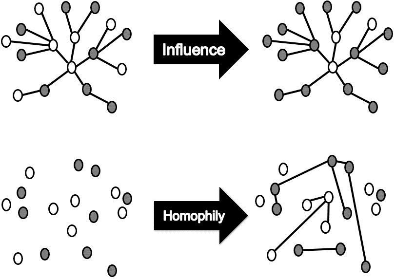
ConfoundingHomophily, andInfluence,. Influence is the process by which an individual (the influential) affects another individual such that the influenced individual becomes more similar to the influential figure. Homophily is observed in already similar individuals. It is realized when similar individuals become friends due to their high similarity. Confounding is environment’s effect on making individuals similar. For instance, individuals who live in Russia, speak Russian fluently due to the environment and are therefore similar in language. The confounding force is an external factor. Confounding is independent of inter-individual interactions and is therefore not discussed further. Note that both influence and homophily social forces give rise to assortative networks. After either of them affects a network, the network exhibits more among similar nodes, but when “friends become similar", we denote that as influence and when “similar individuals become friends", we call it homophily. Figure 8.1 depicts how both influence and homophily affect social networks.
In particular, when discussing influence and homophily in social media, we are interested in asking the following questions:
How can we measure influence or homophily?
How can we model influence or homophily?
How can we distinguish the two?
As both processes result in assortative networks, we can quantify their effect on the network by measuring the assortativity of the network.
8.1 Measuring Assortativity
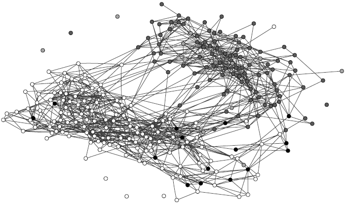
Measuring assortativity helps quantify how much influence, and homophily, among other factors have affected a social network. Assortativity can be quantified by measuring how similar connected nodes are to one another. Figure 8.2 depicts the friendship network in a United States high school in 19941. In the figure, races are represented with different colors: whites are white, blacks are grey, hispanics are light grey, and others are black. As we observe, there is a high assortativity between individuals of the same race. This is observed among whites and also among blacks. Hispanics have a high tendency to become friends with whites.
To measure assortativity, we measure the number of edges that fall in between the nodes of the same race. This technique works for nominal attributes, such as race, but does not work for ordinal ones such as age. Consider a network where individuals are friends with people of different ages. Unlike races, individuals are more likely to be friends with others close in age and not necessarily with ones of the exact same age. Hence, we discuss two techniques: one for nominal attributes and one for ordinal attributes.
8.1.1 Measuring Assortativity for Nominal Attributes
Consider a scenario where we have nominal attributes assigned to nodes. Similar to our aforementioned example, this attribute could be race, nationality, gender, etc. One simple technique to measure assortativity is to consider the number of edges that are between nodes of the same type. Let t(v_i) denote the type of node v_i. In an undirected graph2, G(V,E), with adjacency matrix A, this measure can be computed as follows,
where m is the number of edges in the graph, \frac{1}{m} is applied for normalization, and the factor \frac{1}{2} is added since G is undirected. \delta(.,.) is the Kronecker delta function,
This measure has its own caveats. Consider a school of hispanic students. Obviously, all connections are between hispanics and assortativity value 1 is not a significant finding. However, consider a school where half the population is white and half the population is hispanic. It is statistically expected for 50% of the connections to be between members of different race. If connections in this school were only between whites and hispanics, then it is a significant finding. To account for this issue, we can employ a common technique where we measure the assortativity significance
Assortativity
Significanceby subtracting the measured assortativity by the statistically expected assortativity. The higher this value, the more significant the assortativity observed.
Consider a graph G(V,E), |E| = m, where the degrees are known beforehand (how many friends an individual has), but edges are not. Consider two nodes v_i and v_j, with degrees d_i and d_j, respectively. What is the expected number of edges between these two nodes? Consider node v_i. For any edge going out of v_i randomly, the probability of this edge getting connected to node v_j is \frac{d_j}{\sum_i d_i}=\frac{d_j}{2m}. Since the degree for v_i is d_i, we have d_i such edges; hence, the expected number of edges between v_i and v_j is \frac{d_id_j}{2m}. Now, the expected number of edges between v_i and v_j that are of the same type is \frac{d_id_j}{2m}\delta(~t(v_i),t(v_j)~) and the expected number of edges of the same type in the whole graph is
We are interested in computing the distance between the assortativity observed and the expected assortativity.
This measure is called Modularity
Modularity(Newman 2006). The maximum modularity value for a network depends on the number of nodes of the same type and degree. The maximum occurs when all edges are connecting nodes of the same type, i.e., when A_{ij}=1, \delta (~t(v_i),t(v_j)~)=1. We can normalize modularity by dividing it by the maximum it can take:
Modularity can be simplified using a matrix format. Let \Delta \in \mathbb{R}^{n \times k} denote the indicator matrix and let k denote the number of types,
Note that \delta function can be reformulated using the indicator matrix,
Therefore, (\Delta\Delta^T)_{i,j}=\delta(t(v_i),t(v_j)). Let B= A-\mathbf{d}\mathbf{d}^T/2m denote the modularity matrix where \mathbf{d} \in \mathbb{R}^{n\times 1} is the degree vector for all nodes. Given that the trace of multiplication of two matrices X and Y^T is Tr(XY^T)=\sum_{i,j} X_{i,j}Y_{i,j} and Tr(XY)=Tr(YX), modularity can be reformulated as
Consider the bipartite graph in Figure 8.3:
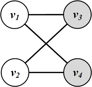
For this bipartite graph,
Therefore, matrix B is
The modularity value Q is
In this example, all edges are between nodes of different color. In other words, the number of edges between nodes of the same color is less than the expected number of edges between them. Therefore, modularity value is negative.
8.1.2 Measuring Assortativity for Ordinal Attributes
A common measure for analyzing the relationship between two variables with ordinal values is covariance
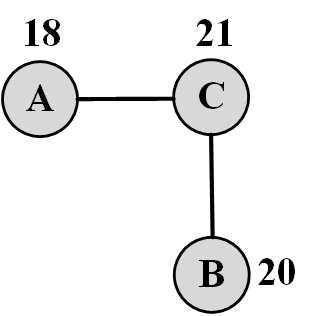
Covariance. Covariance describes how two variables change with respect to each other. In our case, we are interested in how correlated, attribute values of nodes connected via edges are. Let x_i be the ordinal attribute value associated with node v_i. In Figure 8.4, for node c, the value associated is x_c=21.
We construct two variables X_L and X_R, where for any edge (v_i, v_j) we assume that x_i is observed from variable X_L and x_j is observed from variable X_R. For Figure 8.4,
In other words, X_L represents the ordinal values associated with the left node of the edges and X_R represents the values associated with the right node of the edges. Our problem is therefore reduced to computing the covariance between variables X_L and X_R. Note that since we are considering an undirected graph, both edges (v_i, v_j) and (v_j,v_i) exist; therefore, x_i and x_j are observed in both X_L and X_R. Thus, X_L and X_R will include the same set of values but in a different order. This implies that X_L and X_R have the same mean and standard deviation.
Since we have m edges and each edge appears twice for the undirected graph, then X_L and X_R have 2m elements. Each value x_i appears d_i times since it appears as endpoints of d_i edges. The covariance between X_L and X_R is
E(X_L) is the mean (expected value) of variable X_L and E(X_LX_R) is the mean of the multiplication of X_L and X_R. In our our setting and following Equation 8.17, these expectations are as follows,
By plugging Equations 8.23 and 8.24 into Equation 8.22, the covariance between X_L and X_R is
Similar to modularity (Section 1.1.1), we can normalize covariance. PearsonS correlation
Pearson Correlation\rho(X_L,X_R) is the normalized version of covariance,
From Equation 8.18, \sigma(X_L)=\sigma(X_R); thus,
Note the similarity between Equations 8.9 and 8.31. Although modularity is used for nominal and correlation for ordinal attributes, the major difference between the two equations is that the \delta function in modularity is now substituted with x_ix_j in the correlation equation.
Consider Figure 8.4 with values demonstrating the attributes associated with each node. Since this graph is undirected, we have the following edges,
The correlation is between the values associated with the endpoints of the edges. Consider X_L as the value of the left end of an edge and X_R as the value of the right end of an edge,
The correlation between these two variables is \rho(X_L,X_R) = -0.67.
8.2 Influence
Influence 3 is “the act or power of producing an effect without apparent exertion of force or direct exercise of command." In this section, we discuss influence and, in particular, how we can (1) measure influence in social media and (2) design models that concretely detail how individuals influence one another in social media.
8.2.1 Measuring Influence
Influence can be measured based on (1) prediction or (2) observation.
Prediction-based
Influence Measures
Prediction-Based Measures. In prediction-based measurement, we assume that an individual’s attribute or the way she is situated in the network predicts how influential she will be. For instance, we can assume that the gregariousness (e.g., number of friends) of an individual is correlated with how influential she will be. Therefore, it is natural to use any of the centrality measures discussed in Chapter 3 for prediction-based influence measurements. Examples of such centrality measures include PageRank and Degree Centrality. In fact, many of these centrality measures were introduced as influence measuring techniques. For instance, on Twitter, in-degree (number of followers) is a common attribute for measuring influence. Since these methods were covered in-depth in that chapter, in this section we focus on observational techniques.
Observation-Based Measures.
Observation-based
Influence MeasuresIn observation-based measures, we quantify influence of an individual by measuring the amount of influence attributed to the individual. The individuals can influence differently in diverse settings and, depending on the context, the observation-based measuring of influence changes. We detail three different settings and how influence can be measured in each.
When an individual is the role model. This happens in the case of the fashion industry, teachers, celebrities, etc. In this case, the size of the audience that has been influenced due to that fashion, charisma, etc. could act as an accurate measure. A local grade-school teacher has a tremendous influence over a class of students, whereas Gandhi influences millions.
When an individual spreads information. This scenario is more likely when a piece of information, an epidemic, or a product, etc. is being spread in a network. In this case, the size of the cascade, that is the number of hops the information traveled, or the population affected, or the rate at which population gets influenced is considered a measure.
When an individual increases value. As in the case of diffusion of innovations (see Chapter 7), oftentimes when individuals perform actions such as buying a product, they increase the value of the product for other individuals. For example, the first individual who bought a fax machine had no one to send faxes to. The second individual who bought a fax machine increased its value for the first individual. So, the increase (or rate of increase) in the value of an item or action (such as buying a product) is often used as a measure.
Case Studies for Measuring Influence in Social Media
This section provides examples of measuring influence in social media. We discuss measuring influence on the blogosphere and on the micro-blogging site Twitter. These techniques can be adapted to other social media sites, as well.
Measuring social influence on the blogosphere
The goal of measuring influence on the blogosphere is to identify influential bloggers on the blogosphere. Due to the limited time the individuals have, following the influentials is often necessary for fast access to interesting news. One common measure for quantifying influence of bloggers is to use in-degree centrality - the number of (in-)links that points to the blog. Due to the sparsity of in-links, more detailed analysis is required to measure influence in blogosphere.
In their book One American in ten tells the other nine how to vote, where to eat, and what to buy. They are The Influentials (Keller and Berry 2003), Keller and Berry argue that influentials are individuals, there are 1) recognized by others, 2) whose activities result in follow-up activities, 3) have novel perspectives, and 4) are eloquent.
To address these issues, Agarwal et al. (Agarwal et al. 2008) proposed the iFinder system to measure influence for blogposts and identify influential bloggers. In particular, for each one of these four characteristics and a blogpost p, they approximate it by collecting four attributes:
Recognition. Recognition for a blogpost can be approximated by the links that point to the blogpost (in-links). Let \mathcal{I}_p denote the set of in-links that point to blogpost p.
Activity Generation. Activity generated by a blogpost can be estimated using the number of comments that p receives. Let c_p denote the number of comments that blogpost p receives.
Novelty. The blogpost’s novelty is inversely correlated with the number of references a blogpost employs. In particular the more citations a blogpost has, it is considered less novel. Let \mathcal{O}_p denote the set of out-links for blogpost p.
Eloquence. Eloquence can be estimated by the length of the blogpost. Given the informal nature of blogs and the bloggers’ tendency to write short blogposts, longer blogposts are commonly believed to be more eloquent. So, the length of a blogpost l_p can be employed as a measure of eloquence.
Given these approximations for each one of these characteristics, we can design a measure of influence for each blog post. Since the number of out-links inversely affects the influence of a blogpost and in-links increases it, we construct an influence graph, or i-graph, where blogposts are nodes and influence flows through the nodes. The amount of this influence flow
Influence Flowfor each post p can be characterized as
InfluenceFlow(p) = w_{in} \sum_{m=1}^{|\mathcal{I}_p|} {I(P_m)} - w_{out} \sum_{n=1}^{|\mathcal{O}_p|} {I(P_n)},(8.34)where I(.) denotes the influence of a blogpost and w_{in} and w_{out} are the weights that adjust the contribution of in- and out-links, respectively. In this equation, P_m’s are blogposts that point to post p and P_n’s are blogposts that are referred to in post p. Influence flow describes a measure that only accounts for in-links (recognition) and out-links (novelty). To account for the other two factors, we design the influence of a blogpost p as
I(p)=w_{length} l_p(w_{comment}c_p+InfluenceFlow(p)).(8.35)Here, w_{length} is the weight for the length of blogpost4. w_{comment} describes how the number of comments is weighted. Note that the four weights w_{in}, w_{out}, w_{comments}, and w_{length} need to be tuned to make the model more accurate. This tuning can be done by a variety of techniques. For instance, we can use a test-system where the influential posts are already known (labeled data) to tune them. 5 Finally, a blogger’s influence index (iIndex) can be defined as the maximum influence value among all her N blogposts,
iIndex= \max_{p_n \in N} I(p_n).(8.36)Computing iIndex for a set of bloggers over all their blogpost can help identify and rank influential bloggers in a system.
Measuring social influence on Twitter
On Twitter, a micro-blogging platform, users receive tweets from other users by following them. Intuitively, we can think of number of followers as a measure of influence (in-degree centrality). In particular, three measures are frequently utilized for Twitter to quantify influence,
In-degree: the number of users following a person on Twitter. As discussed, the number of individuals who are interested in someone’s tweets, i.e., followers, is commonly used as an influence measure on Twitter. In-degree denotes the “audience size" of an individual.
Number of Mentions: the number of times an individual is mentioned in tweets. Mentioning of an individual with
usernamehandle is performed by including@usernamein a tweet. The number of times an individual is mentioned can be employed as an influence measure. Number of mentions denotes the “ability in engaging others in conversation" (Cha et al. 2010).Number of Retweets: individuals on Twitter have the opportunity to forward tweets to a broader audience via the retweet capability. Clearly, the more one’s tweets are retweeted, the more likely she is influential. Number of retweets indicates individual’s ability in generating content that is worth being passed along.
Each one of these measures by itself can be used to identify influential users in Twitter. This can be performed by utilizing the measure for each individual and then ranking individuals based on their measured influence value. Contrary to public belief, number of followers is considered an inaccurate measure compared to the other two. This is shown in (Cha et al. 2010), where the authors ranked individuals on twitter independently based on these three measures. To see if they are correlated or redundant, they compared ranks of an individuals across three measures using rank correlation measures. One such measure is the Spearman’s rank correlation coefficient
Spearman’s Rank
Correlation,\rho = 1 - \frac{6\sum_{i=1}^{n}(m_1^i-m_2^i)^2}{n^3-n},(8.37)where m_1^i and m_2^i are ranks of individual i based on measures m_1 and m_2, and n is the total number of users. Spearman’s rank correlation is the Pearsons correlation coefficient for ordinal variables that represent ranks (i.e., takes values between 1…n); hence, the value is in range [-1,1]. Their findings suggests that popular users (users with high in-degree) do not necessarily have high ranks in terms of number of retweets or mentions. This can be observed in Table 1.1, which shows the Spearman’s correlation between top 10% influentials for each measure.
Table 8.1: Rank correlation between top 10% of influentials for different measures on Twitter Measures Correlation Value Indegree vs Retweets 0.122 Indegree vs Mentions 0.286 Retweets vs Mentions 0.638
8.2.2 Modeling Influence
In influence modeling, our goal is to design models that can explain how individuals influence one another. Given the nature of social media, it is safe to assume that influence takes place among connected individuals. At times, this network is observable (explicit networks) and at others, unobservable (implicit networks). For instance, in referral networks, where people refer others to join an online service on social media, the network of referrals is often observable. On the other hand, people get influenced to buy products and in most cases, the seller has no information on who referred the buyer, but has approximate estimates on the number of products sold over time. In the observable (explicit) network, we resort to threshold models such as the Linear Threshold Model (LTM)
Linear
Threshold
Model (LTM)to model influence; in implicit networks, we can employ methods such as the Linear Influence Model (LIM) that take the number of individuals who get influenced at different times as input, e.g., the number of buyers per week.
Modeling Influence in Explicit Networks
Threshold models are simple, yet effective methods for modeling influence in explicit networks. In review, in threshold models, nodes make decision based on the number or the fraction (the threshold) of their neighbors that have already decided to make the same decision. Threshold models have been employed in the literature as early as the 1970s in the works of Granovetter and Schelling (Granovetter 1973; Schelling 1971). Using a threshold model, Schelling demonstrated that minor local preferences in having neighbors of the same color leads to global racial segregation.
Linear Threshold Model (LTM) is an example of threshold models. Assume a weighted directed graph where nodes j and i are connected with weight w_{j,i}. This weight denotes how much node j can affect node i’s decision. Due to the possibility of normalizations, without loss of generality we can assume
where N(i) denotes the neighbors of node i. In a linear threshold model, each node i is assigned a threshold \theta_i such that when the amount of influence exerted towards i by its active friends is more than \theta_i, then i becomes active, if still inactive. Thus, for i to become active, we should have
where \mathcal{A} denotes the set of active nodes. The threshold values are generally uniformly assigned to nodes from the interval [0,1]. Note that the threshold \theta_i defines how resistant to change node i is, where a very small \theta_i value might indicate that a small change in the activity of i’s neighborhood results in i becoming active and a large \theta_i shows that i resists changes.
- Require: Graph G(V,E), set of initial activated nodes A_0
- return Final set of activated nodes A_\infty
- i=0;
- Uniformly assign random thresholds \theta_v
- while i=0 or A_{i-1} \neq A_i, i \ge 1 do
- A_{i+1} = A_i
- inactive = V - A_i;
- for all v \in \text{inactive} do
- if \sum_{{j\text{ neighbor of }v}, {j\text{ active}}}w_{j,v} \ge \theta_v. then
- activate v;
- A_{i+1} = A_{i+1} \cup \{v\};
- end if
- end for
- i = i+1;
- end while
- A_\infty = A_i;
- Return A_\infty;
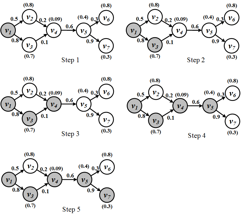
Provided a set of initial active nodes A_0 and a graph, the LTM algorithm is shown in Algorithm 8.1. In each step, for all inactive nodes, the condition in Equation 8.39 is checked and if it is satisfied, the node becomes active. The process ends when no more nodes can be activated. Once \theta thresholds are fixed, the process is deterministic and will always converge to the same state.
Consider the graph in Figure 8.5. Values attached to nodes represent the LTM thresholds and edge values represent the weights. At time 0, node v_1 is activated. At time 2, both nodes v_2 and v_3 receive influence from node v_1. Node v_2 is not activated since 0.5 < 0.8 and node v_3 is activated since 0.8 > 0.7. Similarly, the process continues and at the end, the process stops with 5 activated nodes.
Modeling Influence in Implicit Networks
An implicit network is one where the influence spreads over edges in the network; however, unlike the explicit model, we cannot observe individuals (the influentials) who are responsible for influencing others, but only those who get influenced. In other words, the information available is the set of influenced population P(t) at any time, and the time t_u, when each individual u gets initially influenced (activated). We assume that any influenced individual u can influence I(u,t) number of non-influenced (inactive) individuals at time t. We call I(.,.) the influence function. Assuming discrete time steps, we can formulate the size of influenced population |P(t)|,
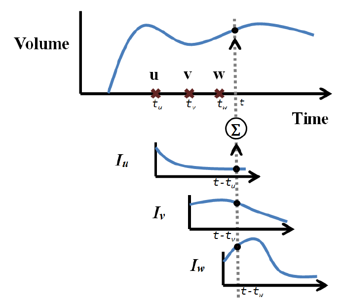
Figure 8.6 demonstrates how the model performs. Individuals u, v, and w are activated at time steps t_u, t_v, and t_w, respectively. At time t, the total number of influenced individuals is a summation of influence functions I_u, I_v, and I_w at time steps t-t_u, t-t_v, and t-t_w, respectively. Our goal is to estimate I(.,.) given activation times and the number of influenced individuals at all times. A simple approach is to utilize a probability distribution to estimate I function. For instance, we can employ the powerlaw distribution to estimate influence. In this case, I(u,t)=c_u(t-t_u)^{-\alpha_u}, where we estimate coefficients c_u and \alpha_u for any u by methods such as maximum likelihood estimation (see (Myung 2003) for more details).
This is called the parametric estimation and the method assumes that all users influence others in the same parametric form. A more flexible approach is to assume a non-parametric function and estimate the influence function’s form. This approach is first introduced as the Linear Influence Model (LIM)
Linear
Influence
Model (LIM)(Yang and Leskovec 2010).
In LIM, we extend our formulation by assuming that nodes get deactivated over time and then no longer influence others. Let A(u,t)=1 denote that node u is active at time t and A(u,t)=0 denote that node u is either deactived or still not influenced. Following a network notation and assuming that |V| is the total size of the population and T is the last time step, we can reformulate Equation 8.40 for |P(t)| as
or equivalently in matrix form,
It is common to assume individuals can only activate other individuals and cannot stop others from becoming activated. Hence, negative values for influence does not make sense; therefore, we would like measured influence values to be positive I\ge 0,
This formulation is similar to regression coefficients computation outlined in Chapter 5, where we compute a least-square estimate of I; however, this formulation cannot be solved using regression techniques we studied earlier since in regression, computed I values can become negative. In practice, this formulation can be solved using non-negative least square methods (see (Lawson and Hanson 1995) for details).
8.3 Homophily
Homophily is the tendency of similar individuals to become friends. It happens on a daily basis in social media and is clearly observable in social networking sites where befriending can explicitly take place. The well-known saying, “birds of a feather flock together" is frequently quoted when discussing homophily. Unlike influence, where an influential influences others, in homophily, two similar individuals decide to get connected.
8.3.1 Measuring Homophily
Homophily is linking of two individuals due to similarity. It leads to assortative networks over time. To measure homophily, we measure how the assortativity of the network has changed over time6. Consider two snapshots of a network G_{t_1}(V,E_{t_1}) and G_{t_2}(V,E_{t_2}) at times t_1 and t_2, respectively, where t_2 > t_1. Without loss of generality, we assume that the number of nodes is fixed and only edges connecting these nodes change, i.e., are added or removed.
When dealing with nominal attributes, the homophily index is defined as
where Q_{normalized} is defined in Equation 8.9. Similarly, for ordinal attributes, the homophily index can be defined as the change in Pearson correlation (Equation 8.31),
8.3.2 Modeling Homophily
Homophily can be modeled using a variation of the Independent Cascade Model discussed in Chapter 7. In this variation, at each time step a single node gets activated and the activated node gets a chance of getting connected to other nodes due to homophily. In other words, if the activated node finds other nodes in the network similar enough (i.e., their similarity is higher than some tolerance value), it connects to them via an edge. A node once activated has no chance of getting activated again.
The algorithm for modeling homophily is outlined in Algorithm 8.2. Let sim(u,v) denote the similarity between nodes u and v. When a node gets activated, we generate a random tolerance value for the node v, between 0 and 1. Alternatively, we can set this tolerance to some predefined value. The tolerance value defines the minimum similarity node v tolerates for connecting to other nodes. Then, for any likely edge (v,u) that is still not in the edge set, if the similarity is sim(v,u) > \theta_v, the edge (v,u) is added. The process continues until all nodes are activated.
- Require: graph G(V,E), E=\emptyset, similarities sim(v,u)
- return Set of Edges E
- for all v \in V do
- \theta_v = generate a random number in [0,1];
- for all (v,u) \not \in E do
- if \theta_v < sim(v,u). then
- E = E \cup {(v,u)};
- end if
- end for
- end for
- Return E;
The model can be used in two different scenarios. First, given a network in which assortativity is attributed to homophily, we can estimate tolerance values for all nodes. To estimate tolerance values, we can simulate the homophily model in Algorithm 8.2 on the given network with different tolerance values and by removing edges. We can compare the assortativity of the simulated network and the given network. By finding the simulated network that best fits the given network (i.e., has closest assortativity value to the given network’s assortativity), we can determine the tolerance values for individuals. Second, when a network is given and the source of assortativity is unknown, we can estimate how much of the observed assortativity can be attributed to homophily. To measure assortativity due to homophily, we can simulate homophily on the given network by removing edges. The distance between the assortativity measured on the simulated network and the given network explains how much of observed assortativity is due to homophily. The smaller this distance the higher the effect of homophily in generating the observed assortativity.
8.4 Distinguishing Influence and Homophily
We are often interested in understanding which social force (influence or homophily) resulted in an assortative network. To distinguish between an influence-based assortativity or homophily-based one, statistical tests can be used. In this section, we discuss three tests: the shuffle test, the edge-reversal test, and the randomization test. The first two can detect whether influence exists in a network or not, but are incapable of detecting homophily. The last one, however, can distinguish influence and homophily. Note that in all these tests, we assume that several temporal snapshots of the dataset are available (like the LIM model) where we know exactly, when each node is activated, when edges are formed, or when attributes are changed.
8.4.1 Shuffle Test
The shuffle test was originally introduced by Anagnostopoulos et al. (Anagnostopoulos et al. 2008). The basic idea behind the shuffle test comes from the fact that influence is temporal. In other words, when u influences v, then v should have been activated after u. So, in shuffle test, we define a temporal assortativity measure. We assume that if there is no influence, then a shuffling of the activation timestamps should not affect the temporal assortativity measurement.
In this temporal assortativity measure, called social correlation
Social Correlation, the probability of activating a node v depends on a, the number of already-active friends she has. This activation probability is calculated using a logistic function 7,
or equivalently,
where \alpha measures the social correlation and \beta denotes the activation bias. For computing the number of already-active nodes of an individual, we need to know the activation timestamps of the nodes.
Let y_{a,t} denote the number of individuals who became activated at time t and had a active friends and let n_{a,t} denote the ones who had a active friends but didn’t get activated at time t. Let y_a=\sum_t y_{a,t} and n_a=\sum_t n_{a,t}. We define the likelihood function as
To estimate \alpha and \beta, we find their values such that the likelihood function denoted in Equation 8.49 is maximized. Unfortunately, there is no closed form solution, but there exist software packages that can efficiently compute the solution to this optimization 8.
The main idea behind the shuffle test is as follows. Let t_u denote the activation time (when a node is first influenced) of node u. When activated-node u influences non-activated node v, and v is activated, then we have t_u < t_v. Hence, when temporal information is available about who activated whom, influenced nodes are activated at a later time than those who influenced them. Now, if there is no influence in the network, we can randomly shuffle the activation time stamps and the predicted \alpha should not change drastically. So, if we shuffle activation time-stamps and predict the correlation coefficient \alpha' and the value of \alpha' is close to the \alpha computed in the original unshuffled dataset, i.e., |\alpha-\alpha'| is small, then the network does not exhibit signs of social influence.
8.4.2 Edge-Reversal Test
The edge reversal test introduced by Christakis and Fowler (Christakis and Fowler 2007) follows a similar approach as shuffle test. If influence resulted in activation then the direction of edges should be important (who influenced whom). So, we can reverse the direction of edges and if there is no social influence in the network, then the value of social correlation \alpha, as defined in Section 1.4.1, should not change dramatically.
8.4.3 Randomization Test
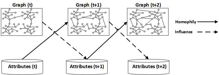
Unlike the other two tests, the randomization test (La Fond and Neville 2010) is capable of detecting both influence and homophily in networks. Let X denote the attributes associated with nodes (age, gender, location, etc.) and X_t denote the attributes at time t. Let X^i denote attributes of node v_i. As mentioned before, in influence, individuals already linked to one another change their attributes, e.g., a user changes habits, whereas in homophily, attributes don’t change but connections are formed due to similarity. Figure 8.7 demonstrates the effect of influence and homophily in a network over time.
The assumption is that if influence or homophily happens in a network, then networks become more assortative. Let A(G_t,X_t) denote the assortativity of network G and attributes X at time t. Then, the network becomes more assortative at time t+1 if
Now, we can assume part of this assortativity is due to influence if the influence gain
Influence Gain and Homophily GainG_{Influence} is positive,
and due to homophily if we have positive homophily gain G_{Homophily},
- Require: G_t, G_{t+1}, X_t, X_{t+1}, number of randomized runs n, \alpha
- return Significance
- g_0=G_{Influence}(t);
- for all 1 \le i \le n do
- X_{t+1}^i=randomize_I(X_t, X_{t+1});
- g_i=A(G_{t},X^i_{t+1})-A(G_{t},X_{t});
- end for
- if g_0 larger than (1-\alpha/2)% of values in \{g_i\}_{i=1}^{n} then
- return significant;
- else if g_0 smaller than \alpha/2% of values in \{g_i\}_{i=1}^{n} then
- return significant;
- else
- return insignificant;
- end if
Note that X_{t+1} denotes the changes in attributes and G_{t+1} denotes the changes in links in the network (new friendships formed). In randomization tests, one determines whether changes in A(G_{t},X_{t+1})-A(G_{t},X_{t}) (influence), or A(G_{t+1},X_{t})-A(G_{t},X_{t}) (homophily) are significant or not. To detect change significance, we use the influence significance test and homophily significance test algorithms outlined in Algorithms 8.3 and 8.4, respectively. The influence significance algorithm
Influence
Significance Teststarts with computing influence gain, which is the assortativity difference observed due to influence (g_0). It then forms a random attribute set at time t+1 (null-hypotheses), assuming that attributes changed randomly at t+1 and not due to influence. This random attribute set X^i_{t+1} is formed from X_{t+1} by making sure that effects of influence in changing attributes are removed.
For instance, assume two users u and v are connected at time t, and u has hobby movies at time t and v does not have this hobby listed at time t. Now, assuming there is an influence of u over v, at time t+1, v adds movies to her set of hobbies. In other words, movies \not\in X^v_t and movies \in X^v_{t+1}. To remove influence, we can remove movies from hobbies of v at time t+1 and add some random hobby such as reading, which is \not\in X^u_t and \not \in X^v_t, to list of hobbies of v at time t+1. This guarantees that the randomized X_{t+1} constructed has no sign of influence. We construct this randomized set n times; this set is then used to compute influence gains \{g_i\}_{i=1}^{n}. Obviously, the more distant g_0 is from these gains, the more significant influence is. We can assume that whenever g_0 is smaller than \alpha/2% (or larger that 1-\alpha/2%) of \{g_i\}_{i=1}^{n} values it is significant. The value of \alpha is set empirically.
- Require: G_t, G_{t+1}, X_t, X_{t+1}, number of randomized runs n, \alpha
- return Significance
- g_0=G_{Homophily}(t);
- for all 1 \le i \le n do
- G_{t+1}^i=randomize_H(G_t, G_{t+1});
- g_i=A(G_{t+1}^i,X_{t})-A(G_{t},X_{t});
- end for
- if g_0 larger than (1-\alpha/2)% of values in \{g_i\}_{i=1}^{n} then
- return significant;
- else if g_0 smaller than \alpha/2% of values in \{g_i\}_{i=1}^{n} then
- return significant;
- else
- return insignificant;
- end if
Similarly, in the homophily significance test
Homophily
Significance Test, we compute the original homophily gain and construct random graph links G^i_{t+1} at time t+1, such that no homophily effect is exhibited in how links are formed. To perform this for any two (randomly-selected) links e_{ij} and e_{kl} formed in the original G_{t+1} graph, we form edges e_{il} and e_{kj} in G^i_{t+1}. This is to make sure that the homophily effect is removed and that the degrees in G^i_{t+1} are equal to that of G_{t+1}.
8.5 Summary
Individuals are driven by different social forces across social media. Two such important forces are influence and homophily.
In influence, an individual’s actions induces her friends to act in a similar fashion. In other words, influence makes friends more similar. Homophily is the tendency for similar individuals to befriend each other. Both influence and homophily result in networks where similar individuals are connected to each other. These are assortative networks. To estimate the assortativity of networks, depending on the attribute type that is tested for similarity, we can employ different measures. We discussed modularity for nominal attributes and correlation for ordinal ones.
Influence can be quantified via different measures. Some are prediction-based, where the measure assumes that some attributes can accurately predict how influential an individual will be, such as with in-degree. Others are observation-based, where the influence score is assigned to an individual based on some history, such as how many he has influenced. We also presented case studies for measuring influence in 1) blogosphere and in 2) Twitter.
Influence can be modeled depending on the visibility of the network. When network information is available, we employ threshold models such as the linear threshold model (LTM) and when network information is not available, we estimate influence rates using the Linear Influence Model (LIM). Similarly, homophily can be measured by computing the assortativity difference in time and can be modeled using a variant of independent cascade models.
Finally, to determine the source of assortativity in social networks, we detail three statistical tests: the shuffle test, the edge-reversal test, and the randomization test. The first two can determine if influence is present in the data and the last one can determine both influence and homophily. All tests require temporal data, where activation times and changes in attributes and links are available.
8.6 Bibliographic Notes
Indications of assortativity observed in real-world can be found in (CURRARINI et al. 2009). General reviews for the assortativity measuring methods discussed in this chapter can be found in (Newman 2003, 2010; Newman and Girvan 2003).
Influence and homophily are extensively discussed in social sciences literature (see (Cialdini and Trost 1998; McPherson et al. 2001)). Interesting experiments in this area can be found in Milgram’s seminal experiment on obedience to authority (Milgram 2009). In his controversial study, Milgram showed many individuals due to fear or to appear cooperative are willing to perform acts that are against their better judgment. He recruited participants in what seemingly looked like a learning experiment. Participants were told that they are supposed to administer increasingly sever electric shocks to another individual (“the learner") if he answers questions incorrectly. These shocks were from 15-450 volts (lethal level). In reality, the learner was a confederate of Milgram, never received any shocks, and was an actor. The actor shouted loudly to demonstrate the painfulness of the shocks. Milgram showed that 65% of participants in his experiments were willing to give lethal electric shocks up to 450 volts to the learner, provided assurance statements such as “Although the shocks may be painful, there is no permanent tissue damage, so please go on", or given direct orders, such as “the experiment requires that you continue." Another study is the recent 32 year longitudinal study on the spread of obesity in social networks (Christakis and Fowler 2007). In this study, Christakis et al. analyze a population of 12,067 individuals. The body mass index for these individuals was available from 1971-2003. They show that an individual’s likelihood of becoming obese over time increased by almost 60% if he or she had an obese friend. This likelihood decreased to around 40% if one had an obese sibling or spouse.
Analyzing influence and homophily is also an active topic in social media mining. For studies regarding Influence and homophily online, refer to (Watts and Dodds 2007; Shalizi and Thomas 2011; CURRARINI et al. 2009; Onnela and Reed-Tsochas 2010; Weng et al. 2010; Bakshy et al. 2011). The effect of influence and homophily on the social network has also been used for prediction purposes. For instance, Tang et al. (Tang et al. 2013) employ the effect of homophily for trust prediction.
Modeling influence is challenging. For a review of threshold models, similar techniques, and challenges, see (Goyal et al. 2010; Watts 2002; Granovetter 1978; Kempe et al. 2003).
In addition to tests discussed for identifying influence or homophily, we refer readers to the works of Aral et al. (Aral et al. 2009) and Snijders et al. (Snijders et al. 2007).
8.7 Exercises
State two common factors that explain why connected people are similar or vice versa.
Measuring Assortativity
What is the range [\alpha_1, \alpha_2] for modularity Q values? Provide examples for both extreme values of the range as well as cases where modularity becomes zero.
What are the limitations for modularity?
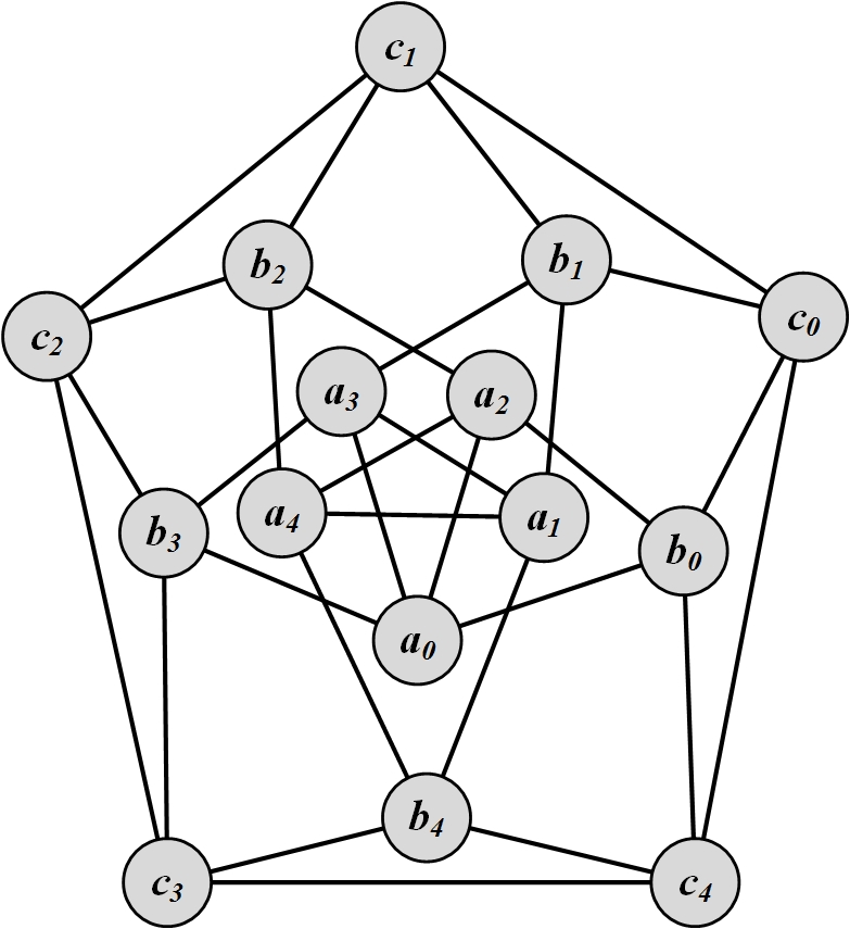
Compute modularity in the following graph. Assume that \{a_i\}_{i=0}^4 nodes are category a, \{b_i\}_{i=0}^4 nodes are category b, and \{c_i\}_{i=0}^4 nodes are category c.
Influence
Does the Linear Threshold Model (LTM) converge? Why?
Follow the LTM procedure until convergence for the following graph. Assume all the thresholds are 0.5 and node X is activated at time 0.
Discuss a methodology for identifying the influentials given multiple influence measures using the following scenario: on Twitter, one can use in-degree and number of retweets as two independent influence measures. How can you find the influentials by employing both measures?
Homophily
Design a measure for homophily that takes into account assortativity changes due to influence.
Distinguishing Influence and Homophily
What is a shuffle test designed for in the context of social influence? Describe how it is performed.
Describe how the edge reversal test works. What is it used for?
From ADD health data: http://www.cpc.unc.edu/projects/addhealth↩︎
The directed case is left to the reader due to minute added complexity.↩︎
As defined by the Merriam-Webster dictionary↩︎
In the original paper, the authors utilize a weight function instead. Here, for clarity, we use coefficients for all parameters.↩︎
Note that Equation 8.35 is defined recursively, since I(p) depends on InfluenceFlow and that, in turn, depends on I(p) (Equation 8.34). Therefore, to estimate I(p), we can use iterative methods where we start with an initial value for I(p) and compute until convergence.↩︎
Note that we have assumed that homophily is the leading social force in the network that leads to its assortativity change. This assumption is often strong for social networks since other social forces act in these networks.↩︎
In the original paper, instead of a, the authors employ \ln (a+1) as the variable. This helps remove the effect of power-law distribution in number of activated friends. Here, for simplicity, we use the non-logarithmic form.↩︎
Note that maximizing this term is equivalent to maximizing the logarithm; this is where Equation 8.48 comes into play.↩︎