Network Measures
In February 2012, Kobe Bryant, the American basketball star, joinedChinese microblogging site Sina Weibo. Within a few hours, more than 100,000 followers joined his page, anxiously waiting for his first microblogging post on the site. The media considered the tremendous number of followers Kobe Bryant received as an indication of his popularity in China. In this case, the number of followers measured Bryant’s popularity among Chinese social media users. In social media, we often face similar tasks in which measuring different structural properties of a social media network can help us better understand individuals embedded in it. Corresponding measures need to be designed for these tasks. This chapter discusses measures for social media networks.
When mining social media, a graph representation is often used. This graph shows friendships or user interactions in a social media network. Given this graph, some of the questions we aim to answer are as follows:
Who are the central figures (influential individuals) in the network?
What interaction patterns are common in friends?
Who are the like-minded users and how can we find these similar individuals?
To answer these and similar questions, one first needs to define measures for quantifying centrality, level of interactions, and similarity, among other qualities. These measures take as input a graph representation of a social interaction, such as friendships (adjacency matrix), from which the measure value is computed.
To answer our first question about finding central figures, we define measures for centrality. By using these measures, we can identify various types of central nodes in a network. To answer the other two questions, we define corresponding measures that can quantify interaction patterns and help find like-minded users. We discuss centrality next.
3.1 Centrality
Centrality defines how important a node is within a network.
3.1.1 Degree Centrality
In real-world interactions, we often consider people with many connections to be important. Degree centrality transfers the same idea into a measure. The degree centrality measure ranks nodes with more connections higher in terms of centrality. The degree centrality C_d for node v_i in an undirected graph is
where d_i is the degree (number of adjacent edges) of node v_i. In directed graphs, we can either use the in-degree, the out-degree, or the combination as the degree centrality value:
Prominence or
Prestige. When using out-degrees, it measures the gregariousness of a node. When we combine in-degrees and out-degrees, we are basically ignoring edge directions. In fact, when edge directions are removed, Equation 3.4 is equivalent to Equation 3.1, which measures degree centrality for undirected graphs.
The degree centrality measure does not allow for centrality values to be compared across networks (e.g., Facebook and Twitter). To overcome this problem, we can normalize the degree centrality values.
Normalizing Degree Centrality
Simple normalization methods include normalizing by the maximumpossible degree,
where n is the number of nodes. We can also normalize by the maximum degree,
Finally, we can normalize by the degree sum,
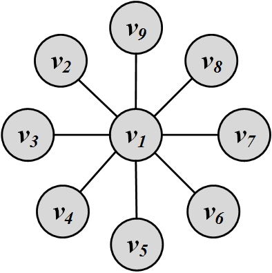
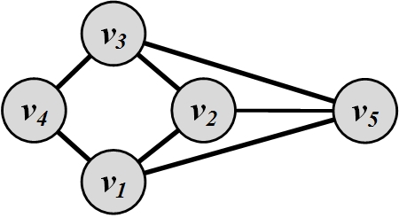
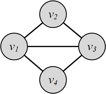
Figure 3.1 shows a sample graph. In this graph, degree centrality for node v_1 is C_d(v_1)=d_{1}=8, and for all others, it is C_d(v_j)=d_j=1, j \neq 1.
3.1.2 Eigenvector Centrality
In degree centrality, we consider nodes with more connections to be more important. However, in real-world scenarios, having more friends does not by itself guarantee that someone is important: having more important friends provides a stronger signal.
Eigenvector centrality tries to generalize degree centrality by incorporating the importance of the neighbors (or incoming neighbors in directed graphs). It is defined for both directed and undirected graphs. To keep track of neighbors, we can use the adjacency matrix A of a graph. Let c_e(v_i) denote the eigenvector centrality of node v_i. We want the centrality of v_i to be a function of its neighbors’ centralities. We posit that it is proportional to the summation of their centralities,
This basically means that \mathbf{C}_e is an eigenvector of adjacency matrix A^T (or A in undirected networks, since A=A^T) and \lambda is the corresponding eigenvalue. A matrix can have many eigenvalues and, in turn, many corresponding eigenvectors. Hence, this raises the question: which eigenvalue–eigenvector pair should we select? We often prefer centrality values to be positive for convenient comparison of centrality values across nodes. Thus, we can choose an eigenvalue such that the eigenvector components are positive.1 This brings us to the
Perron-Frobenius TheoremPerron-Frobenius theorem.
Let A \in \mathbb{R}^{n\times n} represent the adjacency matrix for a [strongly] connected graph or A: A_{i,j} > 0 (i.e. a positive n by n matrix). There exists a positive real number (Perron-Frobenius eigenvalue) \lambda_{\rm max}, such that \lambda_{\rm max} is an eigenvalue of A and any other eigenvalue of A is strictly smaller than \lambda_{\rm max}. Furthermore, there exists a corresponding eigenvector \mathbf{v}=(v_1, v_2, \dots, v_n) of A with eigenvalue \lambda_{\rm max} such that \forall v_i > 0.
Therefore, to have positive centrality values, we can compute the eigenvalues of A and then select the largest eigenvalue. The corresponding eigenvector is \mathbf{C}_e. Based on the Perron-Frobenius theorem, all the components of \mathbf{C}_e will be positive, and this vector corresponds to eigenvector centralities for the graph.
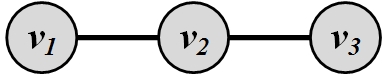
For the graph shown in Figure 3.2(a)(a), the adjacency matrix is
Based on Equation 3.9, we need to solve \lambda \mathbf{C}_e = A \mathbf{C}_e, or
Assuming \mathbf{C}_e=[u_1~u_2~u_3]^T,
Since \mathbf{C}_e \neq [0~0~0]^T, the characteristic equation is
or equivalently,
So the eigenvalues are (-\sqrt{2},0,+\sqrt{2}). We select the largest eigenvalue: \sqrt{2}. We compute the corresponding eigenvector:
Assuming \mathbf{C}_e vector has norm 1, its solution is
which denotes that node v_2 is the most central node and nodes v_1 and v_3 have equal centrality values.
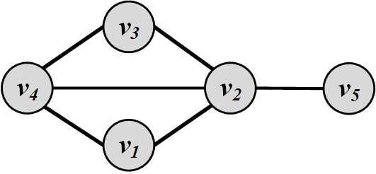
For the graph shown in Figure 3.2(b)(b), the adjacency matrix is as follows:
The eigenvalues of A are (-1.74,-1.27,0.00,+0.33,+2.68). For eigenvector centrality, the largest eigenvalue is selected: 2.68. The corresponding eigenvector is the eigenvector centrality vector and is
Based on eigenvector centrality, node v_2 is the most central node.
3.1.3 Katz Centrality
A major problem with eigenvector centrality arises when it considers directed graphs (see Problem 1 in the Exercises). Centrality is only passed on when we have (outgoing) edges, and in special cases such as when a node is in a directed acyclic graph, centrality becomes zero, even though the node can have many edges connected to it. In this case, the problem can be rectified by adding a bias term to the centrality value. The bias term \beta is added to the centrality values for all nodes no matter how they are situated in the network (i.e., irrespective of the network topology). The resulting centrality measure is called the Katz centrality and is formulated as
The first term is similar to eigenvector centrality, and its effect is controlled by constant \alpha. The second term \beta, is the bias term that avoids zero centrality values. We can rewrite Equation 3.19 in a vector form,
where \mathbf{1} is a vector of all 1’s. Taking the first term to the left hand side and factoring C_{\rm Katz},
Since we are inverting a matrix here, not all \alpha values are acceptable. When \alpha=0, the eigenvector centrality part is removed, and all nodes get the same centrality value \beta. However, once \alpha gets larger, the effect of \beta is reduced, and when \det(\mathbf{I}-\alpha A^T)=0, the matrix \mathbf{I}-\alpha A^T becomes non-invertible and the centrality values diverge
Divergence in
Centrality
Computation. The \det(\mathbf{I}-\alpha A^T) first becomes 0 when \alpha=1/\lambda, where \lambda is the largest eigenvalue2 of A^T. In practice, \alpha < 1/\lambda is selected so that centralities are computed correctly.
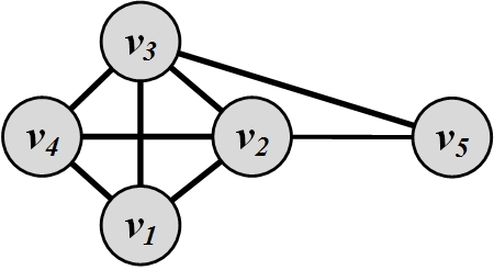
For the graph shown in Figure 3.3, the adjacency matrix is as follows:
The eigenvalues of A are (-1.68, -1.0, -1.0,+0.35,+3.32). The largest eigenvalue of A is \lambda=3.32. We assume \alpha=0.25 < 1/\lambda and \beta=0.2. Then, Katz centralities are
Thus, nodes v_2, and v_3 have the highest Katz centralities.
3.1.4 PageRank
Similar to eigenvector centrality, Katz centrality encounters some challenges. A challenge that happens in directed graphs is that, once a node becomes an authority (high centrality), it passes all its centrality along all of its out-links. This is less desirable, because not everyone known by a well known person is well known. To mitigate this problem, one can divide the value of passed centrality by the number of outgoing links (out-degree) from that node such that each connected neighbor gets a fraction of the source node’s centrality:
This equation is only defined when d_j^{\rm out} is nonzero. Thus, assuming that all nodes have positive out-degrees (d_j^{\rm out} > 0)3, Equation 3.24 can be reformulated in matrix format,
where D = {\it diag}(d_1^{\rm out},d_2^{\rm out},\dots,d_n^{\rm out}) is a diagonal matrix of degrees. The centrality measure is known as the PageRank centrality measure and is used by the
PageRank and Google Web SearchGoogle search engine as a measure for ordering webpages. Webpages and their links represent an enormous web-graph. PageRank defines a centrality measure for the nodes (webpages) in this web-graph. When a user queries Google, webpages that match the query and have higher PageRank values are shown first. Similar to Katz centrality, in practice, \alpha < \frac{1}{\lambda} is selected, where \lambda is the largest eigenvalue of A^T D^{-1}. In undirected graphs, the largest eigenvalue of A^T D^{-1} is \lambda=1; therefore, \alpha < 1.
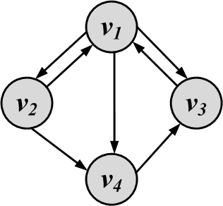
For the graph shown in Figure 3.4, the adjacency matrix is as follows,
We assume \alpha=0.95 < 1 and \beta=0.1. Then, PageRank values are
Hence, nodes v_1 and v_3 have the highest PageRank values.
3.1.5 Betweenness Centrality
Another way of looking at centrality is by considering how important nodes are in connecting other nodes. One approach, for a node v_i, is to compute the number of shortest paths between other nodes that pass through v_i,
where \sigma_{st} is the number of shortest paths from node s to t (also known as information pathways), and \sigma_{st}(v_i) is the number of shortest paths from s to t that pass through v_i. In other words, we are measuring how central v_i’s role is in connecting any pair of nodes s and t. This measure is called betweenness centrality.
Betweenness centrality needs to be normalized to be comparable across networks. To normalize betweenness centrality, one needs to compute the maximum value it takes. Betweenness centrality takes its maximum value when node v_i is on all shortest paths from s to t for any pair (s,t); that is, \forall~(s,t),~s\neq t\neq v_i,~\frac{\sigma_{st}(v_i)}{\sigma_{st}}=1. For instance, in Figure 3.1, node v_1 is on the shortest path between all other pairs of nodes. Thus, the maximum value is
The betweenness can be divided by its maximum value to obtain the normalized betweenness,
Computing Betweenness
In betweenness centrality (Equation 3.29), we compute shortest paths between all pairs of nodes to compute the betweenness value. If an algorithm such as Dijkstra’s is employed, it needs to be run for all nodes, because Dijkstra’s algorithm will compute shortest paths from a single node to all other nodes. So, to compute all-pairs shortest paths, Dijkstra’s algorithm needs to be run |V|-1 times (with the exception of the node for which centrality is being computed). More effective algorithms such as the Brandes’ algorithm (Brandes 2001) have been designed. Interested readers can refer to the bibliographic notes for further references.
For Figure 3.1, the (normalized) betweenness centrality of node v_1 is
Since all the paths that go through any pair (s,t), s \neq t \neq v_1 pass through node v_1, the centrality is 2{8 \choose 2}. Similarly, the betweenness centrality for any other node in this graph is 0.
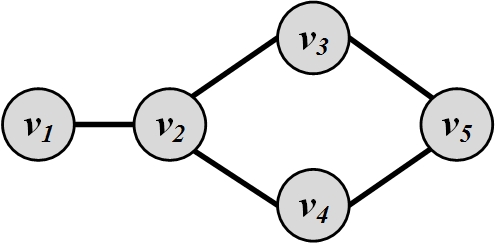
Figure 3.5 depicts a sample graph. In this graph, the betweenness centrality for node v_1 is 0, since no shortest path passes through it. For other nodes, we have
3.1.6 Closeness Centrality
In closeness centrality, the intuition is that the more central nodes are, the more quickly they can reach other nodes. Formally, these nodes should have a smaller average shortest path length to other nodes. Closeness centrality is defined as
where \bar{l}_{v_i}=\frac{1}{n-1}\sum_{v_j\neq v_i}{l}_{i,j} is node v_i\!’s average shortest path length to other nodes. The smaller the average shortest path length, the higher the centrality for the node.
For nodes in Figure 3.5, the closeness centralities are as follows:
Hence, node v_2 has the highest closeness centrality.
The centrality measures discussed thus far have different views on what a central node is. Thus, a central node for one measure may be deemed unimportant by other measures.
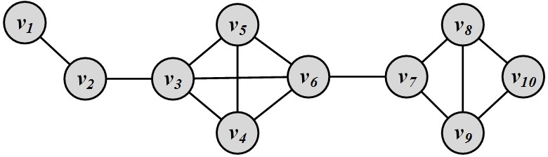
Consider the graph in Figure 3.6. For this graph, we compute the top three central nodes based on degree, eigenvector, Katz, PageRank, betweenness, and closeness centrality methods. These nodes are listed in Table 1.1.
| \mathbf{1^{st}~node} | \mathbf{2^{nd}~node} | \mathbf{3^{rd}~node} | |
|---|---|---|---|
| Degree Centrality | v_3 or v_6 | v_6 or v_3 | v \in \{v_4,v_5,v_7,v_8,v_9\} |
| Eigenvector Centrality | v_6 | v_3 | v_4 or v_5 |
| Katz Centrality: \alpha=\beta=0.3 | v_6 | v_3 | v_4 or v_5 |
| PageRank: \alpha=\beta=0.3 | v_3 | v_6 | v_2 |
| Betweenness Centrality | v_6 | v_7 | v_3 |
| Closeness Centrality | v_6 | v_3 or v_7 | v_7 or v_3 |
As shown in the table, there is a high degree of similarity between most central nodes for the first four measures, which utilize eigenvectors or degrees: degree centrality, eigenvector centrality, Katz centrality, and PageRank. Betweenness centrality also generates similar results to closeness centrality because both use the shortest paths to find most central nodes.
3.1.7 Group Centrality
All centrality measures defined so far measure centrality for a single node. These measures can be generalized for a group of nodes. In this section, we discuss how degree centrality, closeness centrality, and betweenness centrality can be generalized for a group of nodes. Let S denote the set of nodes to be measured for centrality. Let V-S denote the set of nodes not in the group.
Group Degree Centrality
Group degree centrality is defined as the number of nodes from outside the group that are connected to group members. Formally,
Similar to degree centrality, we can define connections in terms of out-degrees or in-degrees in directed graphs. We can also normalize this value. In the best case, group members are connected to all other nonmembers. Thus, the maximum value of C^{\rm group}_d(S) is |V-S|. So dividing group degree centrality value by |V-S| normalizes it.
Group Betweenness Centrality
Similar to betweeness centrality, we can define group betweenness centrality as
Group Closeness Centrality
Closeness centrality for groups can be defined as
One can also use the maximum distance or the average distance to compute this value.
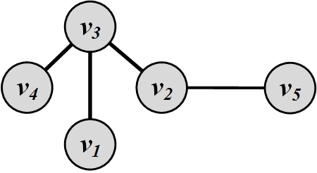
Consider the graph in Figure 3.7. Let S=\{v_2,v_3\}. Group degree centrality for S is
3.2 Transitivity and Reciprocity
Often we need to observe a specific behavior in a social media network. One such behavior is linking behavior. Linking behavior determines how links (edges) are formed in a social graph. In this section, we discuss two well-known measures, transitivity and reciprocity, for analyzing this behavior. Both measures are commonly used in directed networks, and transitivity can also be applied to undirected networks.
3.2.1 Transitivity
In transitivity, we analyze the linking behavior to determine whether it demonstrates a transitive behavior. In mathematics, for a transitive relation R, aRb \wedge bRc \rightarrow aRc. The transitive linking behavior can be described as follows.
Transitive Linking
Let v_1, v_2, v_3 denote three nodes. When edges (v_1, v_2) and (v_2,v_3) are formed, if (v_3,v_1) is also formed, then we have observed a transitive linking behavior (transitivity). This is shown in Figure 3.8.
In a less formal setting,
Transitivity is when a friend of my friend is my friend.
As shown in the definition, a transitive behavior needs at least three edges. These three edges, along with the participating nodes, create a triangle. Higher transitivity in a graph results in a denser graph, which in turn is closer to a complete graph. Thus, we can determine how close graphs are to the complete graph by measuring transitivity. This can be performed by measuring the [global] clustering coefficient and local clustering coefficient. The former is computed for the network, whereas the latter is computed for a node.
Clustering Coefficient
The clustering coefficient analyzes transitivity in an undirected graph. Since transitivity is observed when triangles are formed, we can measure it by counting paths of length 2 (edges (v_1,v_2) and (v_2,v_3)) and checking whether the third edge (v_3,v_1) exists (i.e., the path is closed). Thus, clustering coefficient C is defined as
Alternatively, we can count triangles
Since every triangle has six closed paths of length 2, we can rewrite Equation 3.51 as
In this equation, a triple is an ordered set of three nodes, connected by two (i.e., open triple) or three (closed triple) edges. Two triples are different when
their nodes are different, or
their nodes are the same, but the triples are missing different edges.
For example, triples v_iv_jv_k and v_jv_kv_i are different, since the first triple is missing edge e(v_k,v_i) and the second triple is missing edge e(v_i,v_j), even though they have the same members. Following the same argument, triples v_iv_jv_k and v_kv_jv_i are the same, because both are missing edge e(v_k,v_i) and have the same members. Since triangles have three edges, one edge can be missed in each triple; therefore, three different triples can be formed from one triangle. The number of triangles are therefore multiplied by a factor of 3 in the numerator of Equation 3.52. Note that the clustering coefficient is computed for the whole network.
For the graph in Figure 3.9, the clustering coefficient is
The clustering coefficient can also be computed locally. The following subsection discusses how it can be computed for a single node.
subsubsectionLocal Clustering Coefficient
The local clustering coefficient measures transitivity at the node level. Commonly used for undirected graphs, it estimates how strongly neighbors of a node v (nodes adjacent to v) are themselves connected. The coefficient is defined as
In an undirected graph, the denominator can be rewritten as {d_i \choose 2} = d_i(d_i-1)/2, since there are d_i neighbors for node v_i.
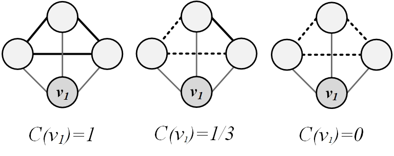
Figure 3.10 shows how the local clustering coefficient changes for node v_1. Thin lines depict v_1’s connections to its neighbors. Dashed lines denote possible connections among neighbors, and solid lines denote current connections among neighbors. Note that when none of the neighbors are connected, the local clustering coefficient is zero, and when all the neighbors are connected, it becomes maximum, C(v_i)=1.
3.2.2 Reciprocity
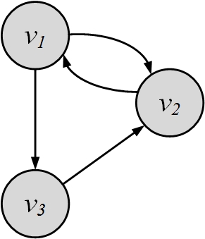
Reciprocity is a simplified version of transitivity, because it considers closed loops of length 2, which can only happen in directed graphs. Formally, if node v is connected to node u, u by connecting to v exhibits reciprocity. On microblogging site Tumblr, for example, these nodes are known as “mutual followers.” Informally, reciprocity is
If you become my friend, I’ll be yours.
Figure 3.11 shows an example where two nodes (v_1 and v_2) in the graph demonstrate reciprocal behavior.
Reciprocity counts the number of reciprocal pairs in the graph. Any directed graph can have a maximum of |E|/2 pairs. This happens when all edges are reciprocal. Thus, this value can be used as a normalization factor. Reciprocity can be computed using the adjacency matrix A:
where {\rm Tr}(A)=A_{1,1} + A_{2,2} + \cdots + A_{n,n}=\sum_{i=1}^{n} A_{i,i} and m is the number of edges in the network. Note that the maximum value for \sum_{i,j} A_{i,j}A_{j,i} is m when all directed edges are reciprocated.
For the graph shown in Figure 3.11, the adjacency matrix is:
Its reciprocity is
3.3 Balance and Status
A signed graph can represent the relationships of nodes in a social network, such as friends or foes. For example, a positive edge from node v_1 to v_2 denotes that v_1 considers v_2 as a friend and a negative edges denotes that v_1 assumes v_2 is an enemy. Similarly, we can utilize signed graphs to represent social status of individuals. A positive edge connecting node v_1 to v_2 can also denote that v_1 considers v_2’s status higher than its own in the society. Both cases represent interactions that individuals exhibit about their relationships. In real-world scenarios, we expect some level of consistency with respect to these interactions. For instance, it is more plausible for a friend of one’s friend to be a friend than to be an enemy. In signed graphs, this consistency translates to observing triads with 3 positive edges (i.e., all friends) more than ones with 2 positive edges and 1 negative edge (i.e., a friend’s friend is an enemy). Assume we observe a signed graph that represents friends/foes or social status. Can we measure the consistency of attitudes that individual have towards one another?
To measure consistency in individual’s attitude, one needs to utilize theories from social sciences to define consistent attitude. In this section, we discuss two theories, social balance and social status, that can help determine consistency in observed signed networks. Social balance is used when edges represent friends/foes and social status is employed when they represent status.
Social Balance Theory, also known as Structural Balance Theory
Structural Balance
Theory, discusses consistency in friend/foe relationships among individuals. Informally, social balance theory says friend/foe relationships are consistent when
The friend of my friend is my friend,
The friend of my enemy is my enemy,
The enemy of my enemy is my friend,
The enemy of my friend is my enemy.
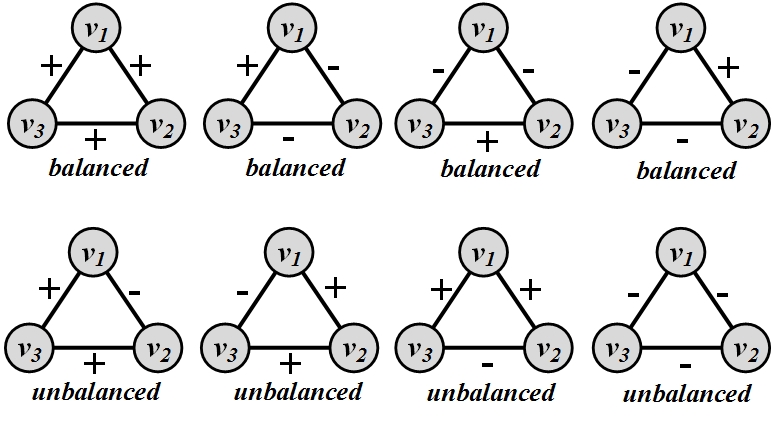
[Sample Graphs for Social Balance Theory. In balanced triangles, we have even number of negative edges.]
We demonstrate a graph representation of social balance theory in Figure 3.12. In this Figure, positive edges demonstrate friendships and negative ones demonstrate enemies. Triangles that are consistent based on this theory are denoted as balanced and triangles that are inconsistent as unbalanced
Balanced and
Unbalanced
Triangles. Let w_{ij} denote the value of the edge between nodes v_i and v_j. Then, for a triangle of nodes v_i, v_j, and v_k, it is consistent based on social balance theory, i.e., it is balanced, if and only if
This is assuming that, for positive edges, w_{ij}=1 and for negative edges, w_{ij}=-1. We observe that, for all balanced triangles in Figure 3.12, the value w_{ij}w_{jk}w_{ki} is positive, and for all unbalanced triangles, it is negative. Social balance can also be generalized to subgraphs other than triangles. In general, for any cycle, if the product of edge values becomes positive, then the cycle is socially balanced.
Social Status Theory. Social status theory measures how consistent individuals are in assigning status to their neighbors. Social status theory can be summarized as
If X has a higher status than Y and Y has a higher status than Z, then X should have a higher status than Z.
We show this theory using two graphs in Figure 3.13. In this Figure, nodes represent individuals. Positive and negative signs show higher or lower status depending on the arrow direction. A directed positive edge from node X to node Y shows that X has a higher status than Y, and a negative one shows vice versa. In the left Figure, v_2 has a higher status than v_1 and v_3 has a higher status than v_2, so based on status theory, v_3 should have a higher status than v_1, but in this graph, we see that v_1 has a higher status in our configuration4. Based on social status theory, this is implausible and thus this configuration is unbalanced. The graph on the right shows a balanced configuration with respect to social status theory.
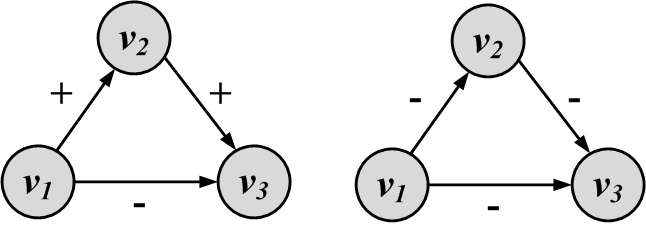
In the example provided in Figure 3.13, social status is defined for the most general example: a set of 3 connected nodes (a triad). However, this can be generalized to other graphs. For instance, in a cycle of n nodes, where n-1 consecutive edges are positive and the last edge is negative, social status considers the cycle balanced.
Note that the same configuration can be considered balanced by social balance theory and unbalanced based on social status theory (see exercises).
3.4 Similarity
In this section we review measures employed to compute similarity between two nodes in a network. In social media, these nodes can represent individuals in a friendship network or products that are related. The similarity between these connected individuals can be either computed based on the network in which they are embedded, i.e., network similarity, or based on the similarity of the content they generate, i.e., content similarity. We discuss content similarity in Chapter 5. In this section, we demonstrate ways to compute similarity between two nodes using network information regarding nodes and edges connecting them. When utilizing network information, the similarity between two nodes can be computed by measuring their structural equivalence or their regular equivalence.
3.4.1 Structural Equivalence
In structural equivalence, we look at the neighborhood shared by two nodes; the size of this neighborhood defines how similar two nodes are. For instance, two brothers have in common sisters, mother, father, grandparents, etc. This shows that they are similar, whereas two random male or female individuals do not have much in common and are not similar.
The similarity measures detailed in this section are based on the overlap between the neighborhoods of the nodes. Let N(v_i) and N(v_j) be the neighbors of nodes v_i and v_j, respectively. In this case, a measure of node similarity can be defined as follows:
For large networks, this value can increase rapidly, since nodes may share many neighbors. Generally, similarity is attributed to a value that is bounded and usually in the range [0,1]. Various normalization procedures can take place such as the
Jaccard Similarity and Cosine SimilarityJaccard similarity or the Cosine similarity,
In general, the definition of neighborhood N(v_i) excludes the node itself (v_i). This leads to problems with the aforementioned similarities because nodes that are connected and do not share a neighbor will be assigned zero similarity. This can be rectified by assuming nodes to be included in their neighborhoods.
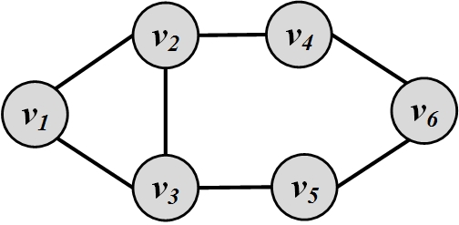
Consider the graph in Figure 3.14. The similarity values between nodes v_2 and v_5 are
A more interesting way of normalizing \sigma(v_i,v_j) is to compare it with the expected value of \sigma(v_i,v_j) when nodes pick their neighbors at random. For nodes v_i and v_j with degrees d_i and d_j, this expectation is \frac{d_id_j}{n}, where n is the number of nodes. This is because there is a \frac{d_i}{n} chance of becoming v_i’s neighbor and, since v_j selects d_j neighbors, the expected overlap is \frac{d_id_j}{n}. We can rewrite \sigma(v_i,v_j) as
Hence, a similarity measure can be defined by subtracting this random expectation:
where \bar{A}_i=\frac{1}{n}\sum_k A_{i,k}. The term \sum_k (A_{i,k}-\bar{A}_{i})(A_{j,k}-\bar{A}_j) is basically the covariance between A_i and A_j. The covariance can be normalized by the multiplication of variances,
which is called the Pearson correlation coefficient
Pearson Correlation. Its value, unlike the other two measures, is in the range [-1,1]. A positive correlation value denotes that when v_i befriends an individual v_k, v_j is also likely to befriend v_k. A negative value denotes the opposite, i.e., when v_i befriends v_k, it is unlikely for v_j to befriend v_k. A zero value denotes that there is no linear relationship between the befriending behavior of v_i and v_j.
3.4.2 Regular Equivalence
In regular equivalence, unlike structural equivalence, we do not look at the neighborhoods shared between individuals, but how neighborhoods themselves are similar. For instance, athletes are similar not because they know each other in person, but since they know similar individuals, such as coaches, trainers, other players, etc. The same argument holds for any other profession or industry since individuals might not know each other in person, but are in contact with very similar individuals. Regular equivalence is defined to assess the similarity by comparing the similarity of neighbors and not by their overlap.
One way of formalizing this is to consider nodes v_i and v_j similar when they have many similar neighbors v_k and v_l. This concept is shown in Figure 3.15(a). Formally,
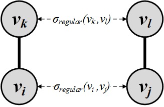
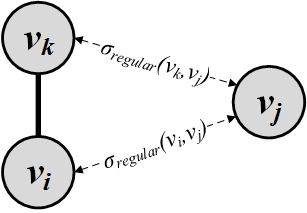
Unfortunately, this formulation is self-referential as solving for i and j requires solving for k and l and solving for k and l requires solving for their neighbors and so on. So, we relax this formulation and assume that node v_i is similar to node v_j when v_j is similar to v_i’s neighbors v_k. This is shown in Figure 3.15(b). Formally,
In vector format, we have
A node is highly similar to itself. To make sure that our formulation guarantees this, we can add an identity matrix to this vector format. Adding an identity matrix will add 1 to all diagonal entries, which represent self-similarities \sigma_{regular}(v_i,v_i):
By rearranging, we get
which we can employ to find the regular equivalence similarity.
Note the similarity between Equation 3.83 and that of Katz centrality (Equation 3.21). Similar to Katz centrality, we must be careful of how to choose \alpha for convergence. A common practice is to select an \alpha such that \alpha < 1/\lambda, where \lambda is the largest eigenvalue of A.
For the graph depicted in Figure 3.14, the adjacency matrix is
The largest eigenvalue of A is 2.43. We set \alpha=0.4 < 1/2.43, and we compute (I-0.4A)^{-1}, which is the similarity matrix
Any row or column of this matrix shows the similarity to other nodes. We can see that node v_1 is most similar (other than itself) to nodes v_2 and v_3. Furthermore, nodes v_2 and v_3 have the highest similarity in this graph.
3.5 Summary
In this chapter, we discuss measures for a social media network. Centrality measures attempt to find the most central node within a graph. Degree centrality assumes that the node with the maximum degree is the most central individual. In directed graphs, prestige and gregariousness are variants of degree centrality. Eigenvector centrality generalizes degree centrality and considers individuals that know many important nodes as central. Based on Perron-Frobenius theorem, eigenvector centrality is determined by computing the eigenvector of the adjacency matrix. Katz centrality solves some of the problems with eigenvector centrality in directed graphs by adding a bias term. PageRank centrality defines a normalized version of Katz centrality. PageRank is used in the Google search engine as a metric to rank web pages. Betweenness centrality assumes that central nodes act as hubs connecting other nodes, and closeness centrality implements the intuition that central nodes are close to all other nodes. Node centrality measures can be generalized to a group of nodes. We discuss group degree centrality, group betweenness centrality, and group closeness centrality.
Linking between nodes (e.g., befriending in social media) is the most commonly observed phenomenon in social media. Linking behavior is analyzed in terms of its transitivity and its reciprocity. Transitivity is “when a friend of my friend is my friend." The transitivity of linking behavior is analyzed by means of clustering coefficient. The global clustering coefficient analyzes this within a network and the local clustering coefficient performs that for a node. Transitivity is commonly considered for closed triads of edges. For loops of length 2, the problem is simplified and is called reciprocity. In other words, reciprocity is when “if you become my friend, I’ll be yours."
To analyze if relationships are consistent in social media, we utilize various social theories to validate outcomes. Social Balance and Social Status are two such theories.
Finally, we analyze node similarity measures. In structural equivalence, two nodes are considered similar when they share neighborhoods. We discuss cosine similarity and Jaccard similarity in structural equivalence. In regular equivalence, nodes are similar when their neighborhoods are similar.
3.6 Bibliographic Notes
General reviews of different measures in graphs, networks, web, and social media can be found in (Newman 2010; Witten et al. 2011; Tan et al. 2006; Jiawei and Kamber 2001; Wassermann and Faust 1994).
A more detailed description of the PageRank algorithm can be found in (Page et al. 1999; Liu 2007). In practice, to compute the PageRank values, Power Iteration Method is used. Power iteration method given a matrix A, produces an eigenvalue \lambda and an eigenvector v of A. In case of PageRank, eigenvalue \lambda is set to 1. The iterative algorithm starts with an initial eigenvector v_0 and then, v_{k+1} is computed from v_{k} as follows,
The iterative process is continued until v_k \approx v_{k+1}, i.e., convergence occurs. Other similar techniques to PageRank for computing influential nodes in a webgraph, such as the HITS (Kleinberg 1999) algorithm can be found in (Chakrabarti 2003; Kosala and Blockeel 2000).Unlike PageRank, the HITS algorithm5 considers two types of nodes: authority nodes and hub nodes. An authority is a webpage that has many in-links. A hub is a page with many out-links. Authority pages have in-links from many hubs. In other words, hubs represent webpages that contain many useful links to authorities and authorities are influential nodes in the webgraph. HITS employs an iterative approach to compute authority and hub scores for all nodes in the graph. Nodes with high authority scores are classified as authorities and nodes with high hub scores as hubs. Webpage with high authority scores or hub scores can be recommended to users in a web search engine.
Betweenness algorithms can be improved using all-pair shortest paths algorithmss (Warshall 1962) or algorithms optimized for computing betweenness, such as the Brandes’ algorithm discussed in (Brandes 2001; Tang and Liu 2010).
A review of node similarity and normalization procedures is provided in (Leicht et al. 2006). Jaccard similarity was introduced in (Jaccard 1901) and Cosine similarity is introduced by Salton (Salton and McGill 1986).
REGE (White 1980, 1984) and CATREGE (Borgatti Martin and Stephen 1993) are well-known algorithms for computing regular equivalence.
3.7 Exercises
~~~~~~~~~~Centrality
Come up with an example of a directed connected graph where eigenvector centrality becomes zero for some nodes. Detail when this happens.
Does \beta have any effect on the order of centralities? In other words, if for one value of \beta the centrality value of node v_i is greater than that of v_j, is it possible to change \beta in a way such that v_j’s centrality becomes larger than that of v_i’s?
In PageRank, what \alpha values can we select in order to guarantee that centrality values are calculated correctly, i.e., values do not diverge?
Calculate PageRank values for this graph when
\alpha = 1, \beta =0
\alpha= 0.85, \beta =1
\alpha= 0, \beta =1
Discuss the effects of different values of \alpha and \beta for this particular problem.
Consider a full n-tree. This is a tree in which every node other than the leaves has n children. Calculate the betweenness centrality for the root node, internal nodes, and leaves.
Show an example where the eigenvector centrality of all nodes in the graph is the same while betweenness centrality gives different values for different nodes.
Transitivity and ReciprocityIn a directed graph G(V,E),
Let p be the probability that any node v_i is connected to any node v_j. What is the expected reciprocity of this graph?
Let m and n be the number of edges and number of nodes, respectively. What is the maximum reciprocity? What is the minimum?
Given all graphs \{~G(V,E)~|~s.t., |E| = m, |V| = n~\},
When m=15 and n=10, find a graph with minimum average clustering coefficient (one is enough).
Can you come up with an algorithm to find such a graph for any m and n?
Balance and Status
Find all conflicting directed triad configurations for social balance and social status. A conflicting configuration is an assignment of positive/negative edge signs for which one theory considers the triad balanced and the other considers it unbalanced.
Similarity
In Figure 3.6,
Compute node similarity using Jaccard and cosine similarity for nodes v_5 and v_4.
Find the most similar node to v_7 using regular equivalence.
This constraint is optional and can be lifted based on the context.↩︎
When \det(\mathbf{I}-\alpha A^T)=0, it can be rearranged as \det(A^T-\alpha^{-1}I)=0, which is basically the characteristic equation. This equation first becomes zero when the largest eigenvalue equals \alpha^{-1}, or equivalently \alpha=1/\lambda.↩︎
When d_j^{\rm out}=0, we know that since the out-degree is zero, \forall i, A_{j,i}=0. This makes the term inside the summation \frac{0}{0}. We can fix this problem by setting d_j^{\rm out}=1 since the node will not contribute any centrality to any other nodes.↩︎
Here, we start from v_1 and follow the edges. One can start from a different node and the result should remain the same.↩︎
HITS stands for Hypertext Induced Topic Search.↩︎