Recommendation in Social Media
Individuals in social media make a variety of decisions on a daily basis. These decisions are about buying a product, purchasing a service, adding a friend, and renting a movie, among others. The individual often faces many options to choose from. These diverse options, the pursuit of optimality, and the limited knowledge that each individual has, creates a desire for external help. At times, we resort to search engines for recommendations; however, the results in search engines are rarely tailored to our particular tastes and are query-dependent, independent of the individuals who search for them.
To ease this process, applications and algorithms are developed to help individuals decide easily, rapidly, and more accurately. These algorithms are tailored to individuals’ tastes such that customized recommendations are available for individuals. These algorithms are called Recommendation Algorithms or Recommender Systems
Recommender System.
Recommender systems are commonly used for product recommendation. Their goal is to recommend products interesting to individuals. Formally, a recommendation algorithm takes a set of users U and a set of items I and learns a function f such that
In other words, the algorithm learns a function that assigns a real value to each user-item pair (u,i), where this value indicates how interested user u is in item i. This value denotes the rating given by user u to item i. The recommendation algorithm is not limited to item recommendation and can be generalized to recommending material, such as people, ads, or content.
Recommendation vs. Search
When individuals seek recommendations, they often utilize web search engines. Search engines are rarely tailored to individuals’ needs and often retrieve the same results as long as the search query stays the same. To receive accurate recommendation from a search engine, one needs to send accurate keywords to the search engine. For instance, the query ‘‘best 2013 movie to watch" issued by an 8-year old and an adult will result in the same set of movies, whereas their individual tastes dictate different movies.
Recommendation systems are designed to recommend individual-based choices. Thus, the same query issued by different individuals result in different recommendations. They commonly employ browsing history, product purchases, user profile information, friends information, etc. to make customized recommendations. As simple as it may look like, a recommendation system algorithm actually has to deal with many challenges.
9.1 Challenges
Recommendation systems face many challenges, some of which are presented next:
Cold Start Problem. Many recommendation systems use historical data or information provided by the user to recommend items, products, etc. However, when individuals join sites, they still haven’t bought any product, or they have no history. This makes it hard to infer what they are going to like when they start on a site. The problem is referred to as the cold-start problem. As an example, consider an online movie rental store. This store has no idea what recently joined users prefer to watch and therefore, can’t recommend something close to their tastes. To address this issue, these sites often ask users to rate a couple of movies before they can recommend others. Some other sites ask users to fill in profile information, such as interests. This information serves as an input to the recommendation algorithm.
Data Sparsity. Similar to the cold-start problem, data sparsity is when not enough historical or prior information is available. Unlike the cold start problem, this is in the system as a whole and is not specific to an individual. In general, data sparsity is due to a few individuals rating many items while many other individuals rate only a few items. Recommender systems often use information provided by other users to help an individual get better recommendations. When this information is not reasonably available, then it is said that a data sparsity problem exists. The problem is more prominent in sites that are recently launched or ones that are not popular.
Attacks. The recommender system is attacked to recommend items otherwise not recommended. For instance, consider a system that recommends items based on similarity between ratings, e.g., lens A is recommended for camera B since they both have rating 4. Now, an attacker that has knowledge of the recommendation algorithm can create a set of fake user accounts and rate lens C (not as good as lens A) highly such that it can get rating 4. This way the recommendation system will recommend C with camera B as well as A. This attack is called push attack
Nuke Attack
and
Push Attack, as it pushes the ratings up such that the system starts recommending items that would otherwise not be recommended. Other attacks such as nuke attacks attempt to stop the whole recommendation system algorithm and make it unstable. A recommendation system should have the means to stop such attacks.Privacy. The more information a recommender system has about the users, the better the recommendations it provides to the users. However, users often avoid revealing information about themselves due to privacy concerns. Recommender systems should address this challenge while protecting individuals’ privacy.
Explanation. Recommendation systems often recommend items without having an explanation for recommending them. For instance, when several items are bought together by many users, the system recommends them to new users. However, the system does not know why these items are bought together. Individuals may prefer some reasons for buying items; therefore, explanation should be provided in recommendation algorithms when possible.
9.2 Classical Recommendation Algorithms
Classical recommendation algorithms have a long history on the web. In recent years, with the emergence of social media sites, these algorithms have been provided with new information, such as friendship information, interactions, etc. We review these algorithms in this section.
9.2.1 Content-Based Methods
Content-based recommendation systems are based on the fact that a user’s interest should match the description of the items that she should be recommended by the system. In other words, the more similar the item’s description to the user’s interest, the higher the likelihood that the user is going to find the item’s recommendation interesting. Content-based recommender systems implement this idea by measuring the similarity between an item’s description to the user’s profile information. The higher this similarity the higher the chance that the item is recommended.
To formalize a content-based method, we first represent both user profiles and item descriptions by vectorizing (see Chapter 5) them using a set of k keywords. After vectorization, item j can be represented as a k-dimensional vector I_j=(i_{j,1},i_{j,2},\dots,i_{j,k}) and user i as U_i=(u_{i,1}, u_{i,2}, \dots, u_{i,k}). To compute the similarity between user i and item j, we can use cosine similarity between the two vectors U_i and I_j,
In content-based recommendation, we compute the top-most similar items to a user j and then recommend these items in the order of similarity. Algorithm 9.1 shows the main steps of content-based recommendation.
- Require: User i's Profile Information, Item descriptions for items j \in \{1, 2, \dots, n\}, k keywords, r number of recommendations.
- return r recommended items.
- U_i=(u_1,u_2, \dots, u_k) = user i's profile vector;
- \{I_j\}_{j=1}^n=(i_{j,1}, i_{j,2}, \dots, i_{j,k})= item j's description vector;
- s_{i,j}=sim({U}_i, {I}_j) ;
- Return top r items with maximum similarity s_{i,j}.
9.2.2 Collaborative Filtering (CF)
Collaborative Filtering is another set of classical recommendation techniques. In collaborative filtering, one is commonly given a user-item matrix where each entry is either unknown or is the rating assigned by the user to an item. Table 1.1 is an user-item matrix where ratings for some cartoons are known and for others, unknown (question marks). For instance, on a review scale of 5, where 5 is the best and 0 is the worst, if an entry (i,j) in the user-item matrix is 4, that means that user i liked item j.
| Lion King | Aladdin | Mulan | Anastasia | |
|---|---|---|---|---|
| John | 3 | 0 | 3 | 3 |
| Joe | 5 | 4 | 0 | 2 |
| Jill | 1 | 2 | 4 | 2 |
| Jane | 3 | ? | 1 | 0 |
| Jorge | 2 | 2 | 0 | 1 |
In collaborative filtering, one aims to predict the missing ratings and possibly recommend the cartoon with the highest predicted rating to the user. This prediction can be performed directly by using previous ratings in the matrix. This approach is called memory-based collaborative filtering since it employs historical data available in the matrix. Alternatively, one can assume that an underlying model (hypothesis) governs the way users rate items. This model can be approximated and learned. After the model is learned, one can use the model to predict other ratings. The second approach is called model-based collaborative filtering.
Memory-Based Collaborative Filtering
In memory-based collaborative filtering, one assumes one of the following (or both) to be true:
Users with similar previous ratings for items are likely to rate future items similarly.
Items that have received similar ratings previously from users are likely to receive similar ratings from future users.
If one follows the first assumption, the memory-based technique is a user-based collaborative filtering algorithm; and if one follows the latter, it is an item-based collaborative filtering algorithm. In both cases, users (or items) collaboratively help filter out irrelevant content (dissimilar users or items). To determine similarity between users or items, in collaborative filtering, two commonly used similarity measures are cosine similarity and Pearson correlation. Let r_{u,i} denote the rating user u assigns to item i and let \bar{r}_u denote the average rating for user u and \bar{r}_i the average rating for item i. Cosine similarity between users i and j is
And the Pearson correlation coefficient is defined as
Next, we discuss user-based collaborative filtering.
User-based Collaborative Filtering. In user-based collaborative filtering, we predict the rating of user u for item i by (1) finding users most similar to u and (2) using a combination of the ratings of these users for item i as the predicted rating of user u for item i. To remove noise and reduce computation, we often limit the number of similar users to some fixed number. These most similar users are called the neighborhood
Neighborhoodfor user u, N(u). In user-based collaborative filtering, the rating of user u for item i is calculated as
where the number of members of N(u) is predetermined, e.g., top 10 most similar members.
In Table 1.1, r_{Jane, Aladdin} is missing. The average ratings are the following:
Using cosine similarity (or Pearson correlation), the similarity between Jane and others can be computed,
Now, assuming that the neighborhood size is 2, then Jorge and Joe are the two most similar neighbors. Then, Jane’s rating for Aladdin computed from user-based collaborative filtering is
Item-based Collaborative Filtering. We discussed user-based collaborative filtering, in which we compute the average rating for different users and compute the most similar users to the users we are seeking recommendations for. Unfortunately, in most online systems, users do not have many ratings; therefore, the averages and similarities may be unreliable. This often results in a different set of similar users when new ratings are added to the system. On the other hand, products usually have many ratings and their average and the similarity between them is more stable. In item-based CF, we perform collaborative filtering by finding most similar items. In item-based collaborative filtering, the rating of user u for item i is calculated as
where \bar{r}_i and \bar{r}_j are the average ratings for items i and j, respectively.
In Table 1.1, r_{Jane, Aladdin} is missing. The average ratings for items are
Using cosine similarity (or Pearson correlation), the similarity between Aladdin and others can be computed,
Now, assuming that the neighborhood size is 2, then Lion King and Anastasia are the two most similar neighbors. Then, Jane’s rating for Aladdin computed from item-based collaborative filtering is
Model-Based Collaborative Filtering
In memory-based methods (either item-based or user-based), one aims to predict the missing ratings based on similarities between users or items. In model-based collaborative filtering, one assumes that an underlying model governs the way users rate. We aim to learn that model and then use that model to predict the missing ratings. Among a variety of model-based techniques, we focus on a well-established model-based technique that is based on Singular Value Decomposition (SVD).
Singular
Value
DecompositionSVD is a linear algebra technique that, given a real matrix X \in \mathbb{R}^{m\times n}, m \ge n, factorizes it into three matrices,
where U \in \mathbb{R}^{m\times m} and V \in \mathbb{R}^{n\times n} are orthogonal matrices and \Sigma \in \mathbb{R}^{m\times n} is a diagonal matrix. The product of these matrices is equivalent to the original matrix; therefore, no information is lost. Hence, the process is lossless
Lossless
Matrix
Factorization.
Let \Vert X \Vert_F = \sqrt{\sum_{i=1}^m \sum_{j=1}^{n} X_{ij}^2} denote the Frobenius norm of matrix X. A low-rank matrix approximation of matrix X is another matrix C \in \mathbb{R}^{m \times n}. C approximates X and C’s rank (the maximum number of linearly independent columns) is a fixed number k << min(m,n)
Frobenius
Norm,
The best low-rank matrix approximation is a matrix C that minimizes \Vert X-C \Vert_F. Low-rank approximations of matrices remove noise by assuming that the matrix is not generated at random and has an underlying structure. SVD can help remove noise by computing a low-rank approximation of a matrix. Consider the following matrix X_k, which we construct from matrix X after computing the SVD of X=U\Sigma V^T:
Create \Sigma_k from \Sigma by keeping only the first k elements on the diagonal. This way, \Sigma_k \in \mathbb{R}^{k \times k}.
Keep only the first k columns of U and denote it as U_k \in \mathbb{R}^{m\times k} and keep only the first k rows of V^T and denote it as {V_k}^T \in \mathbb{R}^{k \times n}.
Let X_k=U_k\Sigma_k {V_k}^T, X_k \in \mathbb{R}^{m \times n}.
As it turns out, X_k is the best low-rank approximation of a matrix X. The following
Eckart-Young-Mirsky
TheoremEckart-Young-Mirsky theorem outlines this result.
Let X be a matrix and C be the best low-rank approximation of X, i.e., \Vert X-C \Vert_F is minimized, and rank(C)=k, then C=X_k.
To summarize, the best rank-k approximation of the matrix can be easily computed by calculating the SVD of the matrix and then taking the first k columns of U, truncating \Sigma to the the first k entries, and taking the first k rows of V^T.
As mentioned, low-rank approximation helps remove noise from a matrix by assuming that matrix is low-rank. By employing this model, we remove noise from the matrix. In low-rank SVD, if X \in \mathbb{R}^{m \times n}, then U_k \in \mathbb{R}^{m \times k}, \Sigma \in \mathbb{R}^{k \times k}, and V^T \in \mathbb{R}^{k \times n}. Hence, U_k has the same number of rows as X, but in a k-dimensional space. Therefore, U represents rows of X, but in a transformed k dimensional space. The same holds for V^T since it has the same number of rows as the number of columns of X, but in a k-dimensional space. To summarize, U and V^T can be thought as k-dimensional representations of rows and columns of X. In this k-dimensional space, noise is removed and hopefully more similar points are closer.
Now, given the user-item matrix X, we can remove its noise by computing X_k from X and get the new k-dimensional user space U or the k-dimensional item space V^T. This way, we can compute the most similar neighbors based on distances in this k-dimensional space. The similarity in the k-dimensional space can be computed using cosine similarity or Pearson correlation. We demonstrate this via Example 9.3.
Consider the following user-item matrix,
| Lion King | Aladdin | Mulan | ||
|---|---|---|---|---|
| John | 3 | 0 | 3 | |
| Joe | 5 | 4 | 0 | |
| Jill | 1 | 2 | 4 | |
| Jorge | 2 | 2 | 0 |
Assuming this matrix is X, then by computing the SVD of X=U\Sigma V^T,1 we have
Considering a rank 2 approximation, i.e., k=2, we truncate all three matrices,
The rows of U_k represent users. Similarly the columns of V^T_k (or rows of V_k) represent items. Thus, we can plot users and items in a 2-D figure. By plotting their columns, we avoid computing distances between them and can visually inspect items or users that are most similar to one another. Figure 9.1 depicts users and items depicted in a 2-D space. As observed in the figure, to recommend for Jill, John is the most similar individual. Similarly, the most similar item to Lion King is Aladdin.
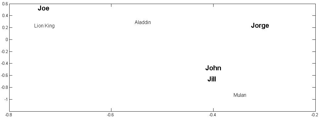
After most similar items or users are found in the lower k-dimensional space, one can follow the same process outlined in user-based or item-based collaborative filtering to find the ratings for an unknown item. For instance, we observed in Example 9.3 (see Figure 9.1) that if we are predicting the rating r_{Jill, Lion King} and assume neighborhood size is 1, item-based CF uses r_{Jill, Aladdin}, since Aladdin is closest to Lion King. Similarly, user-based collaborative filtering uses r_{John, Lion King}, since John is the closest user to Jill.
9.2.3 Extending Individual Recommendation to Groups of Individuals
All methods discussed thus far are used to predict rating for item i for an individual u. Advertisements individuals receive via email marketing are examples of this type of recommendation on social media. However, consider ads displayed on the starting page of a social media site. These ads are shown to a large population of individuals. The goal when showing these ads is to ensure that they are interesting to the individuals who observe them. In other words, we are advertising to a group of individuals.
Our goal is to formalize how existing methods for recommending to a single individual can be extended to a group of individuals. Consider a group of individuals G=\{u_1,u_2,\dots, u_n\} and a set of products I=\{i_1,i_2,\dots, i_m\}. From the products in I, we aim to recommend products to our group of individuals G such the recommendation satisfies the group being recommended to as much as possible. One approach to recommending for the group of individuals is to first consider the ratings predicted for each individual in the group and then devise methods that can aggregate ratings for the individuals in the group. Products that have the highest aggregated ratings are selected for recommendation. Next, we discuss these aggregation strategies for individuals in the group.
Aggregation Strategies for a Group of Individuals
We discuss three major aggregation strategies for individuals in the group. Each aggregation strategy considers an assumption based on which ratings are aggregated. Let r_{u,i} denote the rating of user u \in G for item i \in I. Denote R_i, the group aggregated rating, for item i.
Maximizing Average Satisfaction. We assume that products that satisfy each member of the group on average are the best to be recommended to the group. Then, R_i group rating based on the maximizing average satisfaction strategy is given as
After we compute R_i for all items i \in I, we recommend the items that have the highest R_i’s to members of the group.
Least Misery. This strategy combines ratings by taking the minimum of them. In other words, we want to guarantee that no individuals is being recommended an item that he or she strongly dislikes. In least misery, the aggregated rating R_i of an item is given as
Similar to the previous strategy, we compute R_i for all items i \in I and recommend the items with the highest R_i values. In other words, we prefer recommending items to the group such that no member of the group strongly dislikes the item.
Most Pleasure. Unlike the least misery strategy, in most pleasure, we take the maximum rating in the group as the group rating:
Since we recommend items that have highest R_i values, this strategy guarantees that the items that are being recommended to the group are enjoyed the most by at least one member of the group.
Consider the following user-item matrix. Consider group G=\{John, Jill, Juan\}. For this group, the aggregated ratings for all products using average satisfaction, least misery, and maximum pleasure are as follows.
| Soda | Water | Tea | Coffee | |
|---|---|---|---|---|
| John | 1 | 3 | 1 | 1 |
| Joe | 4 | 3 | 1 | 2 |
| Jill | 2 | 2 | 4 | 2 |
| Jorge | 1 | 1 | 3 | 5 |
| Juan | 3 | 3 | 4 | 5 |
Average Satisfaction:
Least Misery:
Maximum Pleasure:
Thus, the first recommended items are Tea, Water, and Coffee based on Average Satisfaction, Least Misery, and Maximum Pleasure, respectively.
9.3 Recommendation using Social Context
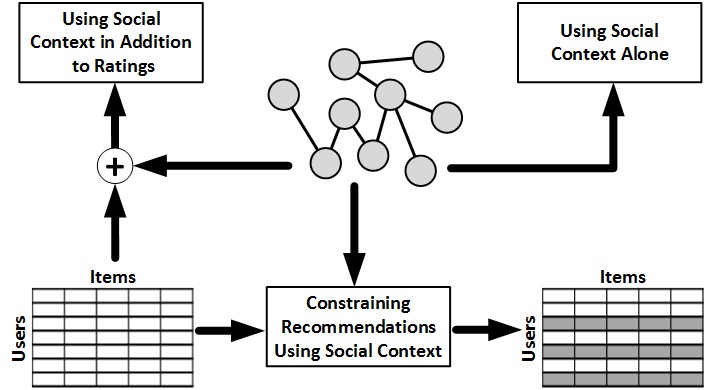
In social media, in addition to ratings of products, there is additional information available, such as the friendship network among individuals. This information can be utilized to improve recommendations. When utilizing this friendship network, we assume that an individual’s friends have impact on the ratings ascribed to the individual. This can be due to homophily, influence, or confounding, discussed in Chapter 8. When utilizing this social information, i.e., Social Context, we can (1) use friendship information alone, (2) use social information in addition to ratings, or (3) constrain recommendations using social information. Figure 9.2 compactly represents these three approaches.
9.3.1 Utilizing Social Context Alone
Consider a network of friendships for which no user-item rating matrix is provided. In this network, we can still recommend users from the network to other users for friendship. This is an example of friend recommendation in social networks. For instance, in social networking sites, users are often provided with a list of individuals they may know and are asked if they wish to befriend them. How can we recommend such friends?
There are many methods that can be utilized to recommend friends in social networks. One such method is Link Prediction, which we discuss in detail in Chapter 10. We can also utilize the structure of the network to recommend friends. For example, it is well known that individuals often form triads of friendships on social networks. In other words, two friends of an individual are often friends with one another. A triad of three individuals a, b, and c consists of three edges e(a,b), e(b,c), and e(c,a). A triad that is missing one of these edges is denoted as an open triad. To recommend friends, we can find open triads and recommend individuals that are not connected as friends to one another.
9.3.2 Extending Classical Methods with Social Context
Social information can also be utilized in addition to a user-item rating matrix to improve recommendation. Addition of social information can be performed by assuming that users that are connected (i.e., friends) have similar tastes in rating items. We can model taste of user U_i using a k-dimensional vector U_i \in \mathbb{R}^{k \times 1}. We can also model items in the k-dimensional space. Let V_j \in \mathbb{R}^{k\times 1} denote the item representation in k-dimensional space. We can assume that rating R_{ij} given by user i to item j can be computed as
To compute U_i and V_i, we can utilize matrix factorization. We can rewrite Equation 9.52 in matrix format as
where R \in \mathbb{R}^{n\times m}, U \in \mathbb{R}^{k\times n}, V \in \mathbb{R}^{k\times m}, n is the number of users, and m is the number of items. Similar to model-based CF discussed in 1.2.2.2, matrix factorization methods can be utilized to find U and V, given user-item rating matrix R. In mathematical terms, in this matrix factorization, we are finding U and V by solving the following optimization problem:
Users often have only a few ratings for items; therefore, R matrix is very sparse and has many missing values. Since we compute U and V only for non-missing ratings, we can change Equation 9.54 to
where I_{ij} \in \{0,1\} and I_{ij}=1 when user i has rated item j and is equal to 0 otherwise. This ensures that non-rated items do not contribute to the summations being minimized in Equation 9.55. Often, when solving this optimization problem, the computed U and V can estimate ratings for the already rated items accurately but fail at predicting ratings for unrated items. This is known as the overfitting problem
Overfitting. The overfitting problem can be mitigated by allowing both U and V to only consider important features required to represent the data. In mathematical terms, this is equivalent to both U and V having small matrix norms. Thus, we can change Equation 9.55 to
where \lambda_1,\lambda_2 >0 are predetermined constants that control the effects of matrix norms. The terms \frac{\lambda_1}{2}||U||^2_F and \frac{\lambda_2}{2}||V||^2_F are denoted as regularization terms
Regularization
Term. Note that to minimize Equation 9.56, we need to minimize all terms in the equation, including the regularization terms. Thus, whenever one needs to minimize some other constraint, it can be introduced as a new additive term in Equation 9.56. Equation 9.56 lacks a terms that incorporates the social network of users. For that, we can add another regularization term
where sim(i,j) denotes the similarity between user i and j (e.g., cosine similarity or Pearson correlation between their ratings) and F(i) denotes the friends of i. When this terms is minimized, it ensures that the taste for user i is close to all his friends j \in F(i). Similar to previous regularization terms, we can add this term to Equation 9.55. Hence, our final goal is to solve the following optimization problem:
where \beta is the constant that controls the effect of social network regularization. A local minimum for this optimization problem can be solved 9.58 using gradient-descent based approaches. To solve this problem, we can compute the gradient with respect to U_i’s and V_i’s and perform a gradient-descent-based method.
9.3.3 Recommendation Constrained by Social Context
In classical recommendation, to estimate ratings of an item, one determines similar users or items. In other words, any user similar to the individual can contribute to the predicted ratings for the individual. We can limit the set of individuals that can contribute to the ratings of a user to the set of friends of the user. For instance, in user-based collaborative filtering, we determine a neighborhood of most similar individuals. We can take the intersection of this neighborhood with the set of friends of the individual to attract recommendations only from friends who are similar enough:
This approach has its own shortcomings. When there is no intersection between the set of friends and the neighborhood of most similar individuals, the ratings cannot be computed. To mitigate this, one can utilize the set of k most similar friends of an individual S(i) to predict the ratings,
Similarly, when friends are not very similar to the individual, the predicted rating can be different from the rating predicted using most similar users. Depending on the context, both equations can be utilized.
Consider the following user-item matrix and the adjacency matrix denoting the friendship among these individuals.
| Lion King | Aladdin | Mulan | Anastasia | |
|---|---|---|---|---|
| John | 4 | 3 | 2 | 2 |
| Joe | 5 | 2 | 1 | 5 |
| Jill | 2 | 5 | ? | 0 |
| Jane | 1 | 3 | 4 | 3 |
| Jorge | 3 | 1 | 1 | 2 |
We wish to predict r_{Jill, Mulan}. We compute the average ratings and similarity between Jill and other individuals using cosine similarity.
The similarities are
Considering a neighborhood of size 2, the most similar users to Jill are John and Jane, i.e.,
We also know that friends of Jill are
We can utilize Equation 9.59 to predict the missing rating by taking the intersection of friends and neighbors.
Similarly, we can utilize Equation 9.60 to compute the missing rating. Here, we take Jill’s 2 most similar neighbors: Jane and Jorge.
9.4 Evaluating Recommendations
When a recommendation algorithm predicts ratings for items, one must evaluate how accurate its recommendations are. One can evaluate the (1) accuracy of predictions, (2) relevancy of recommendations, or (3) rankings of recommendations.
9.4.1 Evaluating Accuracy of Predictions
When evaluating the accuracy of predictions, we measure how close predicted ratings are to the true ratings. Similar to the evaluation of supervised learning, we often predict the ratings of some items with known ratings (i.e., true ratings) and compute how close the predictions are to the true ratings. One of the simplest methods, Mean Absolute Error (MAE) computes the average absolute difference between the predicted ratings and true ratings,
where n is the number of predicted ratings, \hat{r}_{ij} is the predicted rating, and r_{ij} is the true rating. Normalized Mean Absolute Error (NMAE) normalizes MAE by dividing it by the range ratings can take,
where r_{\max} is the maximum rating among all rated items and r_{\min} is the minimum. In MAE, error linearly contributes to the MAE value. We can increase this contribution by considering summation of squared errors in Root Mean Squared Error (RMSE):
Consider the following table with both the predicted ratings and true ratings of 5 items:
| Item | Predicted Rating | True Rating |
|---|---|---|
| 1 | 1 | 3 |
| 2 | 2 | 5 |
| 3 | 3 | 3 |
| 4 | 4 | 2 |
| 5 | 4 | 1 |
The MAE, NMAE, and RMSE values are
9.4.2 Evaluating Relevancy of Recommendations
When evaluating recommendations based on relevancy, we ask users if they find the recommended items relevant to their interests. Given a set of recommendations to a user, the user describes each recommendation as relevant or irrelevant. Based on the selection of items for recommendations and their relevancy, we can have the four types of items outlined in Table 1.5. Given this table, we can define measures that utilize relevancy information provided by users. Precision is one such measure. It defines the fraction of relevant items among recommended items.
| Selected | Not Selected | Total | |
|---|---|---|---|
| Relevant | N_{rs} | N_{rn} | N_{r} |
| Irrelevant | N_{is} | N_{in} | N_{i} |
| Total | N_{s} | N_{n} | N |
Similarly, we can utilize recall to evaluate a recommender algorithm, which provides the probability of selecting a relevant item for recommendation.
We can also combine both precision and recall by taking their harmonic mean in F-Measure.
Consider the following recommendation relevancy matrix for a set of 40 items. For this table, the precision, recall, and F-measure values are
| Selected | Not Selected | Total | |
|---|---|---|---|
| Relevant | 9 | 15 | 24 |
| Irrelevant | 3 | 13 | 16 |
| Total | 12 | 28 | 40 |
9.4.3 Evaluating Ranking of Recommendations
Often, we predict ratings for multiple products for a user. Based on the predicted ratings, we can rank products based on their levels of interestingness to the user. This ranking can be evaluated. Given the true ranking of interestingness of items, we can compare this ranking with it and report a value. Rank correlation measures the correlation between the predicted ranking and the true ranking. One such technique is the Spearman’s rank correlation discussed in Chapter 8. Let x_i, 1 \le x_i \le n, denote the rank predicted for item i, 1 \le i \le n. Similarly, let y_i, 1 \le y_i \le n, denote the true rank of item i from the user’s perspective. Spearman’s rank correlation is defined as
where n is the total number of items.
Here, we discuss another rank correlation measure: Kendall’s tau. We say that the pair of items (i,j) are concordant
Kendall’s Tauif their ranks \{x_i,y_i\} and \{x_j,y_j\} are in order:
A pair of items is discordant if their corresponding ranks are not in order:
When x_i=x_j or y_i=y_j, the pair is neither concordant nor discordant. Let c denote the total number of concordant item pairs and d the total number of discordant item pairs. Kendall’s tau computes the difference between the two, normalized by the total number of item pairs {n \choose 2}:
Kendall’s tau takes value in range [-1,1]. When the ranks completely agree, all pairs are concordant and Kendall’s tau takes value 1, and when the ranks completely disagree, all pairs are discordant and Kendall’s tau takes value -1.
Consider a set of 4 items I=\{i_1,i_2,i_3,i_4\} for which the predicted and true rankings are as follows:
| Predicted Rank | True Rank | |
|---|---|---|
| i_1 | 1 | 1 |
| i_2 | 2 | 4 |
| i_3 | 3 | 2 |
| i_4 | 4 | 3 |
The pair of items and their status {concordant/discordant} are
Thus, Kendall’s tau for the rankings is
9.5 Summary
In social media, recommendations are constantly being provided. Friend recommendation, product recommendation, and video recommendation, among others, are all examples of recommendations taking place in social media. Unlike web search, recommendation is tailored to individuals’ interests and can help recommend more relevant items. Recommendation is challenging due to the cold start problem, data sparsity, attacks on these systems, privacy concerns, and the need for an explanation on why items are being recommended.
In social media, sites often resort to classical recommendation algorithms to recommend items or products. These techniques can be divided into content-based methods and collaborative filtering techniques. In content-based methods, we utilize the similarity between the content (e.g., item description) of items and user profiles to recommend items. In collaborative filtering (CF), we utilize historical ratings of individuals in the form of a user-item matrix to recommend items. CF methods can be categorized into memory-based and model-based techniques. In memory-based techniques, we utilize the similarity between users (user-based) or items (item-based) to predict missing ratings. In model-based techniques, we assume that an underlying model describes how users rate items. Using matrix factorization techniques we approximate this model, using which, missing ratings can be predicted. Classical recommendation algorithms often predict ratings for individuals. We discuss ways to extend these techniques to groups of individuals.
In social media, we can also utilize friendship information to give recommendations. These friendships alone can help recommend (e.g., friend recommendation), can be added as complementary information to classical techniques, or can be utilized to constrain the recommendations provided by classical techniques.
Finally, we discuss evaluation of recommendation techniques. Evaluation can be performed in terms of accuracy, relevancy, and rank of recommended items. We discuss MAE, NMAE, and RMSE from methods that evaluate accuracy, precision, recall, and F-measure from relevancy-based methods, and Kendall’s tau from rank-based methods.
9.6 Bibliographic notes
General references for the content provided in this chapter can be found in (Jannach et al. 2010; Resnick and Varian 1997; Schafer et al. 1999; Adomavicius and Tuzhilin 2005). In social media, recommendation is utilized for various items, including blogs (Arguello et al. 2008), news (Liu et al. 2010; Das et al. 2007), videos (Davidson et al. 2010), and tags (Sigurbjörnsson and Van Zwol 2008), among others. For example, YouTube video recommendation system employs co-visitation counts to compute the similarity between videos (items). To perform recommendations, videos with high similarity to a seed set of videos are recommended to the user. The seed set consists of the videos users watched on YouTube (beyond a certain threshold), as well as videos that are explicitly favorited, “liked", rated, or added to playlists.
Among classical techniques, more on content-based recommendation can be found in (Pazzani and Billsus 2007) and more on collaborative filtering can be found in (Su and Khoshgoftaar 2009; Sarwar et al. 2001; Schafer et al. 2007). Content-based and CF methods can be combined into hybrid methods which are not discussed in this chapter. A survey of hybrid methods is available in (Burke 2002). More details on extending classical techniques to groups is discussed in (Jameson and Smyth 2007).
When recommending using social context, we can utilize additional information such as tags (Guy et al. 2010; Sen et al. 2009) or trust (Golbeck and Hendler 2006; O’Donovan and Smyth 2005; Massa and Avesani 2004; Ma et al. 2009). For instance, in (Tang, Gao, and Liu 2012), the authors discern multiple facets of trust and apply multi-faceted trust in social recommendation. In another work, Tang et al. (Tang, Gao, Liu, and Sarma 2012), exploit the evolution of both rating and trust relations for social recommendation. Users in the physical world are likely to ask for suggestions from their local friends while they also tend to seek suggestions from users with high global reputations (e.g., reviews by vine voice reviewers of Amazon.com). Therefore, in addition to friends, one can also use global network information for better recommendations. In (Tang et al. 2013), the authors exploit both local and global social relations for recommendation.
When recommending people (potential friends), we can utilize all these types of information. A comparison between different people recommendation techniques can be found the work of Chen et al. (Chen et al. 2009). Methods that extend classical techniques with social context are discussed in (Ma et al. 2011, 2008; Konstas et al. 2009).
9.7 Exercises
~~~~~~~~~~Classical Recommendation Algorithm
Discuss one difference between content-based recommendation and collaborative filtering.
Compute the missing rating using user-based collaborative filtering (CF). Use cosine similarity to find the nearest neighbors.
God Father Le Cercle Rouge Cidade de Deu Rashomon La vita e bella \bar{r}_u Newton 3 0 3 3 2 Einstein 5 4 0 2 3 Gauss 1 2 4 2 0 Aristotle 3 ? 1 0 2 1.5 Euclid 2 2 0 1 5 Assuming that you have computed similarity values in the following table, calculate Aristotle’s rating by completing these 4 tasks:
Calculate the similarity value between Aristotle and Einstein;
Identify Aristotle’s 2 nearest neighbors;
Calculate \bar{r}_u values for everyone (Aristotle’s is given); and
Calculate Aristotle’s rating for “Le Cercle Rouge".
Newton Einstein Gauss Euclid Aristotle 0.76 ? 0.40 0.78 In an item-based nearest-neighbor recommendation, describe how the recommender finds and recommends items to the given user.
Recommendation Using Social Context
Provide two examples where social context can help improve classical recommendation algorithms in social media.
In Equation 9.58, the term \beta\sum_{i=1}^n\sum_{j \in F(i)}\sigma(i,j)||U_i-U_j||^2_F is added to model the similarity between friends’ tastes. Let T \in \mathbb{R}^{n\times n} denote the pairwise trust matrix, in which 0 \le T_{ij} \le 1 denotes how much user i trusts user j. Using your intuition on how trustworthiness of individuals should affect recommendations received from them, modify Equation 9.58 using trust matrix T.
Evaluating Recommendation Algorithms
What does “high precision" mean? Why is precision alone insufficient to measure performance under normal circumstances? Provide an example to show that both precision and recall are important.
When is Kendall’s tau equal to -1? In other words, how is the predicted ranking different from the true ranking?
In Matlab, this can be performed using the
svdcommand↩︎