Information Diffusion in Social Media
In February 2013, during the third quarter of Super Bowl XLVII, a power outage stopped the game for 34 minutes. Oreo, a sandwich cookie company, tweeted during the outage: “Power out? No Problem, You can still dunk it in the dark". The tweet caught on almost immediately, reaching nearly 15,000 retweets and 20,000 likes on Facebook in less than 2 days. A simple tweet diffused into a large population of individuals. It helped the company gain fame with minimum budget in an environment where companies spent as much as 4 million dollars to run a 30 second ad during the super bowl. This is an example of Information Diffusion.
This chapter discusses information diffusion in social media. Information diffusion is studied in a plethora of sciences. We discuss methods from fields such as sociology, epidemiology, and ethnography, which can help social media mining. Our focus is on techniques that can model information diffusion.
Societies provide means for information exchange among individuals. Information is exchanged is through various channels. For instance, people share knowledge with their immediate network (friends) or broadcast via public media (TV, newspaper, etc.) throughout the society. Given this flow of information, different research fields have disparate views of what an information diffusion process is. We define information diffusion as the process by which a piece of information (knowledge) is spread and reaches individuals through interactions. The diffusion process involves the following
Sender(s). A sender or a small set of senders that initiate the information diffusion process;
Receiver(s). A receiver or a set of receivers that receive diffused information. Commonly, the set of receivers is much larger than the set of senders and can overlap with the set of senders; and
Medium. This is the medium through which the diffusion takes place. For example, when a rumor is spreading, the medium can be the personal communication between individuals.
This definition can be generalized to other domains. In a disease spreading process, the disease is the analog to the information and infection can be considered a diffusing process. The medium in this case is the air shared by the infecter and the infectee. A diffusion of innovations process can be interrupted. We define the process of interfering with information diffusion by expediting, delaying, or even stopping diffusion as Intervention
Intervention.
Individuals in online social networks are situated in a network, where they interact with others. This network is at times unavailable or unobservable. The information diffusion process takes place in this network. Individuals facilitate information diffusion by making individual decisions that allow information to flow. For instance, when a rumor is spreading, individuals decide if they are interested in spreading it to their neighbors. This decision is performed either dependently (i.e., depending on information of others) or independently. When dependent decisions are taken, it is important to gauge the level of dependence individuals have on others. This could be local dependence, where an individual’s decision is dependent on all her immediate neighbors (friends) or global dependence, where all individuals in the network are observed before making decisions
Local and Global
Dependence.
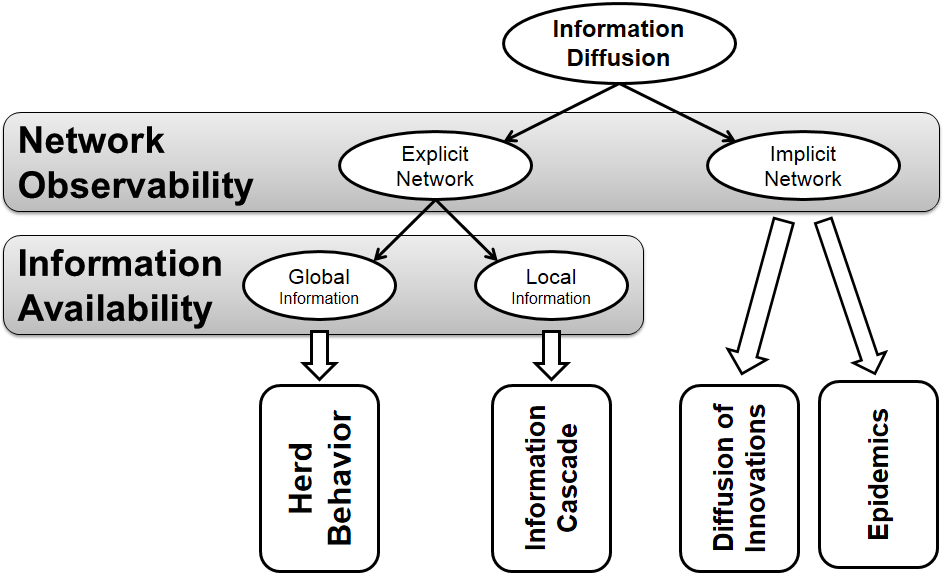
Following our discussion, we detail four general types of information diffusion: Herd Behavior, Information Cascades, Diffusion of Innovation, and Epidemics.
Herd behavior takes place when individuals observe actions of all others and act in an aligned form with them. An information cascade describes the process of diffusion when individuals merely observe their immediate neighbors. In information cascades and herd behavior, the network of individuals is observable; however, in herding, individuals decide based on global information (global dependence), whereas, in information cascades, decisions are taken based on immediate neighbors (local dependence).
Diffusion of innovations provides a bird’s eye view of how an innovation (e.g., a product, music video, or fad) spreads through a population. It assumes that interactions among individuals are unobservable, and the sole available information is the rates at which products are being adopted throughout a certain period of time. This is particularly interesting for companies performing market research, where the sole available information are the rates at which their products are being bought. These companies have no access to interactions among individuals. Epidemic models are similar to diffusion of innovations models, with the difference that the innovation’s analog is a pathogen and adoption is replaced by infection. Another difference is that in epidemic models, individuals don’t decide on getting infected and infection is considered a random natural process, as long as the individual is exposed to the pathogen. Figure 7.1 summarizes our discussion by providing a decision tree of the information diffusion types.
7.1 Herd Behavior
Consider people participating in an online auction. In this case, individuals can observe the behavior of others by monitoring the bids that are being placed on different items. Individuals are connected via the auction’s site where they can not only observe the bidding behaviors of others, but can also often view profiles of others to get a feel for their reputation and expertise. In these online auctions, it is common to observe individuals participating actively in auctions, where the item being sold might otherwise be considered unpopular. This is due to individuals trusting others and assuming that the high number of bids that the item has received is a strong signal of its value. In this case, Herd Behavior has taken place.
Herd behavior, first coined by British surgeon Wilfred Trotter (Trotter 1916), describes when a group of individuals performs actions that are aligned without previous planning. This has been observed in flocks, herds of animals, and in humans during sporting events, demonstrations, and religious gatherings, to name a few. In general, any herd behavior requires two components:
Connections between individuals; and
A method to transfer behavior among individuals or to observe their behavior.
Individuals can also make decisions that are aligned with others (mindless decisions) when they conform to social or peer pressure. A well-known example is the set of experiments performed by Solomon Asch during the 1950s (Asch 1956)
Solomon Asch
Conformity
Experiment. In one experiment, he asked groups of students to participate in a vision test where they were shown two cards (Figure 7.2), one with a single line segment and one with 3 lines, and the participants were required to match line segments with the same length.
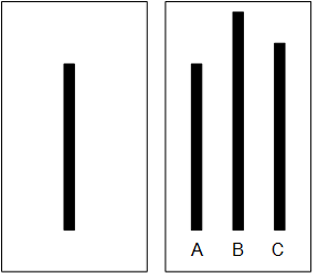
Each participant was put into a group where all other group members were collaborators with Asch. These collaborators were introduced as participants to the subject. Asch found that in control groups with no pressure to conform, only 3% of the subjects provided an incorrect answer. However, when participants were surrounded by individuals providing an incorrect answer, up to 32% of the responses were incorrect.
Unlike this experiment, we refer to the process in which individuals consciously make decisions aligned with others by observing the decisions of other individuals as herding or herd behavior. In theory, there is no need to have a network of people. In practice, there is a network and this network is close to a complete graph, where nodes can observe at least most other nodes. We provide an example of herd behavior that follows our definition.
Diners Example (Banerjee 1992). Assume you are on a trip in a metropolitan area that you are less familiar with. Planning for dinner, you find restaurant A with excellent reviews online and decide to go there. When arriving at A, you see A is almost empty and restaurant B, which is next door and serves the same cuisine, almost full. Deciding to go to B, based on the belief that other diners have also had the chance of going to A, is an example of herd behavior.
In this example, when B is getting more and more crowded, herding is taking place. Herding happens since we consider crowd intelligence trustworthy. We assume that there must be private information not known to us, but known to the crowd, that resulted in the crowd preferring restaurant B over A. In other words, we assume that given this private information, we would have also chosen B over A.
In general, when designing a herding experiment, the following 4 conditions need to be satisfied:
There needs to be a decision made. In our examples, they are going to a restaurant or predicting majority color;
Decisions need to be in sequential order;
Decisions are not mindless and people have private information that helps them decide; and
No message passing is possible. Individuals don’t know the private information of others, but can infer what others know from what is observed from their behavior.
A similar example has been provided by Anderson and Holt (Anderson and Holt 1996, 1997) where students guess whether an urn containing red and blue marbles is majority red or majority blue. Each student has access to the guesses of students beforehand. Anderson and Holt observed a herd behavior where students reached a consensus regarding the majority color over time. It has been shown (Easley and Kleinberg 2010) that Bayesian modeling is an effective technique for demonstrating why this herd behavior occurs. Simply put, students computing conditional probabilities and selecting the most probable majority color results in herding over time. We detail this experiment and how conditional probabilities can explain why herding takes place next.
7.1.1 Bayesian Modeling of Herd Behavior
In this section, we discuss how Bayesian modeling can be utilized to explain herd behavior. We detail the urn experiment, introduced by Anderson and Holt (Anderson and Holt 1996, 1997). In a large class of students, we have an urn that has three marbles in it. These marbles are either blue (B) or red (R) and we are guaranteed to have at least one of each. So, the urn is either majority blue (B,B,R) or majority red (R,R,B). We assume the probability of being either majority blue or majority red is 50%. During the experiment, each student comes to the urn, picks one marble, and checks its color in private. The student predicts majority blue or red, writes her prediction on the blackboard, and puts the marble back in the urn. Students can’t see the color of the marble taken out and can only see the predictions made by different students regarding the majority color on the board. Before students start, the board is clear. Let BOARD variable denote the sequence of predictions written on the blackboard. So, before the first student,
We start with the first student. If the marble selected is red, the prediction will be majority red, otherwise majority blue. Assuming it was blue, on the board we have
The second student can observe a blue or a red marble. If blue, he also predicts majority blue since he knows that the previous student must have observed blue. If red, then he knows that since he has observed red and the first student has observed blue, so he can randomly assume majority red or blue. So, after the second student we either have
Assume we end up with BOARD: {B, B}. In this case, if the third student takes out a red ball, the conditional probability is higher for majority blue, although he observed a red marble. Hence, a herd behavior takes place, and on the board, we will have BOARD: {B,B,B}. From this student and onward, independent of what is being observed, everyone will predict majority blue. Let us demonstrate why this happens based on conditional probabilities and our problem setting. In our problem, we know that the first student predicts majority blue if P(\text{majority blue}|\textit{student's obervation})>1/2 and majority red otherwise. We also know from the experiments setup that
Let us assume that the first student observes blue; then,
Therefore, P(\text{majority blue}|blue)=\frac{2/3\times 1/2}{1/2}=2/3. So, if the first student observes blue, she will predict majority blue, and if she observes red, she will predict majority red. Assuming the first student observes blue, The same argument holds for the second student; if blue is observed, he will also predict majority blue. Now, in the case of the third student, assuming she has observed red, and having BOARD: {B,B} on the blackboard, then,
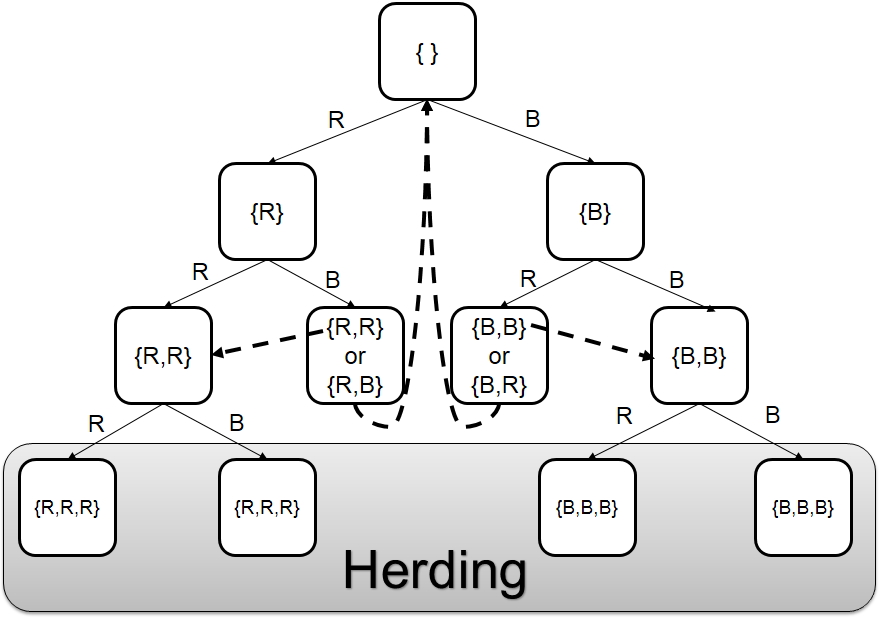
Therefore, P(\text{majority blue}|blue,blue,red)=\frac{4/27\times 1/2}{1/9}=2/3. So, the third student predicts majority blue even though she observes red. Any student after the third student also predicts majority blue regardless of what is being observed since the conditional remains above 1/2. Note that the urn can in fact be majority red. For instance, when blue,blue,red is observed, there is a 1/3 \times 1/3 \times 2/3=2/27 chance that it is majority red; however, due to herding, the prediction could become incorrect. Figure 7.3 depicts the herding process. In the figure, rectangles represent the board status and edge values represent the observations. Dashed arrows depict transitions between states that contain the same statistical information to the students.
7.1.2 Intervention
As herding converges to a consensus over time, it is interesting how one can intervene with this process. In general, intervention is possible by providing private information to individuals not previously available. Consider an urn experiment where individuals decide on majority red over time. Either 1) a private message to individuals informing them that the urn is majority blue or 2) writing the observations next to predictions on the board stops the herding and changes decisions.
7.2 Information Cascades
In social media, individuals commonly repost content posted by others in the network. This content is often received via immediate neighbors (friends). An Information Cascade occurs as information propagates through friends.
Formally, an information cascade is defined as a piece of information or decision being cascaded among a set of individuals, where 1) individuals are connected by a network and 2) individuals are only observing decisions of their immediate neighbors (friends). Therefore, cascade users have less information available to them compared to herding users, where almost all information about decisions are available.
There are many approaches to modeling information cascades. Next, we introduce a basic model that can help explain information cascades.
7.2.1 Independent Cascade Model (ICM)
In this section, we discuss the Independent Cascade Model (ICM) (Kempe et al. 2003) that can be utilized to model information cascades. Variants of this model have been discussed in the literature. Here, we discuss the one detailed by Kempe et al. (Kempe et al. 2003). Interested readers can refer to bibliographic notes for further references. Underlying assumptions for this model include the following:
The network is represented using a directed graph. Nodes are actors and edges depict the communication channels between them. A node can only influence nodes that it is connected to;
Decisions are binary - nodes can be either active or inactive. An active nodes means that the node decided to adopt the behavior, innovation, or decision;
A node, once activated, can activate its neighboring nodes; and
Activation is a progressive process, where nodes change from inactive to active, but not vice versa 1.
Considering nodes that are active as senders and nodes that are being activated as receivers, in the independent cascade model (ICM) senders activate receivers. Therefore, ICM is denoted as a sender-centric
Sender-Centric
Modelmodel. In this model, the node that becomes active at time t, in the next time step t+1, has one chance of activating each of its neighbors. Let v be an active node at time t. Then, for any neighbor w, there is a probability p_{v,w} that node w gets activated at t+1. A node v that has been activated at time t has a single chance of activating its neighbor w and that activation can only happen at t+1. We start with a set of active nodes and we continue until no further activation is possible. Algorithm 7.1 details the process of the ICM model.
- Require: Diffusion graph G(V,E), set of initial activated nodes A_0, activation probabilities p_{v,w}
- return Final set of activated nodes A_\infty
- i=0;
- while i=0 or A_{i-1} \neq A_i, i \ge 1 do
- A_{i+1} = A_i
- i = i+1;
- active = A_i;
- for all v \in \text{active} do
- for all w neighbor of v do
- rand = generate a random number in [0,1];
- if rand < p_{v,w} then
- activate w;
- A_{i+1} = A_{i+1} \cup \{w\};
- end if
- end for
- end for
- end while
- A_\infty = A_i;
- Return A_\infty;
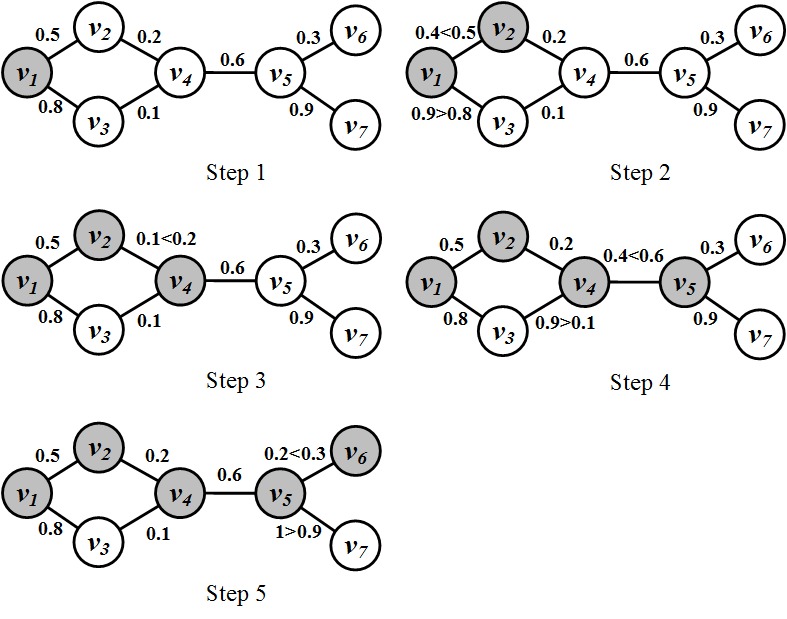
Consider the network in Figure 7.4 as an example. The network is undirected; therefore, we assume p_{v,w}=p_{w,v}. Since it is undirected, for any two vertices connected via an edge, there is an equal chance of one activating the other. Consider the network in step 1. The values on the edges denote p_{v,w}’s. The ICM procedure starts with a set of nodes activated. In our case, it is node v_1. Each activated node gets one chance of activating its neighbors. The activated node generates a random number for each neighbor. If the random number is less than the respective p_{v,w} of the neighbor (see Algorithm 7.1 - lines 9-11), the neighbor gets activated. The random numbers generated are shown in Figure 7.4 in the form of inequalities, where the left hand side is the random number generated and the right hand side is the p_{v,w}. As depicted, by following the procedure after 5 steps, 5 nodes get activated and the ICM procedure converges.
Clearly, the independent cascade model characterizes an information diffusion process 2. It is sender-centered and once a node is activated, it aims to activate all its neighboring nodes. Node activation in ICM is a probabilistic process. Thus, we might get different results for different runs.
One interesting question when dealing with the ICM model is that given a network, how can we activate a small set of nodes initially such that the final number of activated nodes in the network is maximized? We discuss this next.
7.2.2 Maximizing the Spread of Cascades
Consider a network of users and a company that is marketing a product. The company is trying to advertise its product in the network. The company has a limited budget; therefore, not all users can be targeted. However, when users find the product interesting, they can talk with their friends (immediate neighbors) and market the product. Their neighbors, in turn, will talk about it with their neighbors and as this process progresses, the news about the product is spread to a population of nodes in the network. The company plans on selecting a set of initial users such that the size of the final population talking about the product is maximized.
Formally, let S denote a set of initially activated nodes (seed set) in ICM. Let f(S) denote the number of nodes that get ultimately activated in the network if nodes in S are initially activated. For our ICM example depicted in Figure 7.4, |S|=1 and f(S)=5. Given a budget k, our goal is to find a set S such that its size is equal to our budget |S|=k and f(S) is maximized.
Since the activations in ICM depend on the random number generated for each node (see line 9, Algorithm 7.1), it is challenging to determine the number of nodes that ultimately get activated f(S), for a given set S. In other words, the number of ultimately activated individuals can be different depending on the random numbers generated. ICM can be made deterministic (non-random) by generating these random numbers in the beginning of the ICM process for the whole network. In other words, we can generate a random number r_{u,w} for any connected pair of nodes. Then, whenever node v has a chance of activating u, instead of generating the random number, it can compare r_{u,w} with p_{v,w}. Following this approach, ICM becomes deterministic and given any set of initially activated nodes S, we can compute the number of ultimately activated nodes f(S).
Before finding S, we detail properties of f(S). The function f(S) is non-negative since for any set of nodes S, in the worst case, no node gets activated; hence, it is non-negative. It is also monotone:
This is because when a node is added to the set of initially activated nodes, it either increases the number of ultimately activated nodes or keeps them the same. Finally, f(S) is submodular
Submodular
function. A set function f is submodular if for any finite set N,
The proof that function f is submodular is beyond the scope of this book, but interested readers are referred to (Kempe et al. 2003) for the proof. So, f is non-negative, monotone, and submodular. Unfortunately, for a submodular non-negative monotone function f, finding a k element set S such that f(S) is maximized is an NP-Hard problem (Kempe et al. 2003). In other words, we know no efficient algorithm for finding this set 3. Often, when a computationally challenging problem is at hand, approximation algorithms come in handy. In particular, the following theorem helps us approximate S.
(Kempe et al. 2003) Let f be a 1) non-negative, 2) monotone, and 3) submodular set function. Construct k-element set S, each time by adding node v, such that f(S \cup \{v\}) is maximized. Let S^{Optimal} be the k-element set such that f is maximized. Then f(S) \ge (1-\frac{1}{e})f(S^{Optimal}).
This theorem states that by constructing the set S greedily one can get at least a (1-1/e)\approx 63\% approximation of the optimal value. Algorithm 7.2 details this greedy approach. The algorithm starts with an empty-set S and adds node v_1, which ultimately activates most other nodes if activated. Formally, v_1 is selected such that f(\{v_1\}) is the maximum. The algorithm then selects the second node v_2 such that f(\{v_1,v_2\}) is maximized. The process is continued until the k^{\text{th}} node v_k is selected. Following this algorithm, we find an approximately reasonable solution for the problem of cascade maximization.
- Require: Diffusion graph G(V,E), budget k
- return Seed set S (set of initially activated nodes)
- i=0;
- S=\{\};
- while i \neq k do
- v = \arg \max_{v \in V\setminus S} f(S \cup \{v\});
- S= S \cup \{v\};
- i=i+1;
- end while
- Return S;
For the following graph, assume that node i activates node j when |i-j| \equiv 2~(mod~3). Solve cascade maximization for k=2.
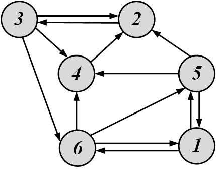
To find the first node v, we compute f(\{v\}) for all v. We start with node 1. At time 0, node 1 can only activate node 6, since
At time 1, node 1 can no longer activate others, but node 6 is active and can activate others. Node 6 has outgoing edges to nodes 4 and 5. From 4 and 5, node 6 can only activate 4,
At time 2, node 4 is activated. It has a single outlink to node 2 and since |4-2| \equiv 2~(mod~3), 2 is activated. Node 2 cannot activate other nodes; therefore, f(\{1\})=4. Similarly, we find that f(\{2\})=1, f(\{3\})=1, f(\{4\})=2, f(\{5\})=1, and f(\{6\})=4. So, 1 or 6 can be chosen for our first node. Let us choose 6. If 6 is initially activated, nodes 1,2,4, and 6 will become activated at the end. Now, from the set \{1,2,3,4,5,6\} \setminus \{1,2,4,6\}=\{3,5\}, we need to select one more node. We have f(\{3\})=f(\{5\})=1, so we can select one node randomly. We choose 3. So, S=\{6,3\}.
7.2.3 Intervention
Consider a false rumor spreading in social media. This is an example where we are interested in stopping an information cascade in social media. Intervention in independent cascade model can be achieved via 3 possible methods:
By limiting the number of outlinks of the sender-node and potentially reducing the chance of activating others. Note that when the sender node is not connected to others via directed edges, no one will get activated by the sender.
By limiting the number of in-links of receiver nodes and therefore reducing their chance of getting activated by others.
By increasing the activation probability of a node (p_{v,w}) and therefore reducing the chance of activating others.
7.3 Diffusion of Innovations
Diffusion of innovations is a phenomenon observed regularly in social media. A music video getting viral or a piece of news being retweeted many times are examples of innovations diffusing across social networks. As defined by Rogers, an innovation is "an idea, practice, or object that is perceived as new by an individual or other unit of adoption" (Rogers 1995). Innovations are created regularly; however, not all innovations spread through populations. The theory of diffusion of innovations aims to answer why and how these innovations spread. It also describes the reasons behind the diffusion process, individuals involved, as well as the rate at which ideas spread. In this section, we review characteristics of innovations that are likely to be diffused through populations and detail well-known models in the diffusion of innovations. Finally, we provide mathematical models that can model the process of diffusion of innovations, and how we can intervene with these models.
7.3.1 Innovation Characteristics
For an innovation to be adopted, the individual adopting it (adopter) and the innovation must encompass certain qualities.
Innovations must be highly observable, should have relative advantage to current practices, should be compatible with the socio-cultural paradigm to which being presented, should be observable under various trials (trialability), and should not be highly complex.
For individual characteristics, it has been observed by many researchers (Rogers 1995; Hirschman 1980) that the adopter should be earlier in adopting the innovation, compared to other members of her social circle (innovativeness).
7.3.2 Diffusion of Innovations Models
Some of the earliest models for diffusion of innovations were provided by Gabriel Tarde in the early 20th century (Tarde 1907). We review basic diffusion of innovations models. Interested readers may refer to bibliographical notes for further study.
Ryan and Gross - Adopter Categories
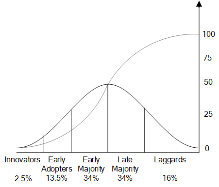
Ryan and Gross studied the adoption of hybrid seed corn by farmers in Iowa (Strang and Soule 1998; Ryan and Gross 1943). The hybrid seed corn was highly resistant to diseases and other catastrophes such as droughts. However, farmers did not adapt it due to its price and the seed’s inability to reproduce. Their study showed that farmers received information through two main channels: one being mass communications from companies selling the seeds and the other being interpersonal communications with other farmers. They found that although farmers received information from the mass channel, the influence was coming from the interpersonal channel. They argued that adoption depended on a combination of both. They also observed that the adoption rate follows an S-shaped curve and that there are 5 different types of adopters based on the order that they adopt the innovations, namely: 1) textitInnovators (top 2.5%), 2) Early Adopters (13.5%), 3) Early Majority (34%), 4) Late Majority (34%), and 5) Laggards (16%). Figure 7.6 depicts the distribution of these adopters as well as the cumulative adoption S-shaped curve. As shown in the figure, the adoption rate is slow when innovators or early adopters adopt the product. Once early majority individuals start adopting, the adoption curve becomes linear and the rate is constant until all late majority members adopt the product. After the late majority adopts the product, the adoption rate becomes slow once again when laggards start their adoption, and the curve slowly approaches 100%.
Katz - Two-Step Flow Model
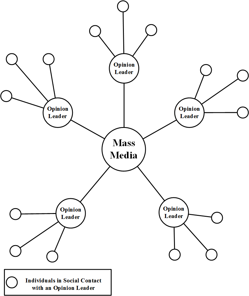
Elihu Katz, a professor of communication at the University of Pennsylvania, is a well-known figure in the study of the flow of information. In addition to a study similar to the hybrid corn seed on how physicians adopted the new tetracycline drug (Coleman et al. 1966), Katz also developed a two-step flow model (also known as the multi-step flow model) (Katz and Lazarsfeld 2006) that describes how information is delivered through mass communication. The basic idea is depicted in Figure 7.7. Most information comes from mass media, which is then directed towards influential figures called opinion leaders. These leaders then convey the information (or form opinions) and act as hubs for other members of the society.
Rogers - Diffusion of Innovations Process
Rogers in his well-known book, Diffusion of Innovations (Rogers 1995), discusses various theories regarding the diffusion of innovations process. In particular, he describes a five stage process of adoption:
Awareness: in this stage, the individual becomes aware of the innovation, but her information regarding the product is limited;
Interest: the individual shows interest in the product and seeks more information;
Evaluation: the individual tries the product in his mind and decides whether or not to adopt it;
Trial: the individual performs a trial use of the product; and
Adoption: the individual decides to continue the trial and adopts the product for full use.
7.3.3 Modeling Diffusion of Innovations
To effectively make use of the theories in the diffusion of innovations, we demonstrate a mathematical model for it in this section. The model incorporates basic elements discussed up till now and can be used to effectively model a diffusion of innovations process. This model can be concretely described as
Here, A(t) denotes the total population that adopted the innovation till time t. i(t) denotes the coefficient of diffusion, which describes the innovativeness of the product being adopted, and P denotes the total number of potential adopters (till time t). This equation shows that the rate at which number of adopters changes throughout time depends on how innovative the product being adopted is. The adoption rate only affects the potential adopters that have not yet adopted the product. Since A(t) is the total population of adopters till time t, it is a cumulative sum and can be computed as follows:
where a(t) defines the adopters at time t. Let A_0 denote the number of adopters at time t_0. There are various methods of defining the diffusion coefficient (Mahajan 1985). One way is to define i(t) as a linear combination of the cumulative number of adopters at different times A(t),
where \alpha_i’s are the weights for each time step. Often a simplified version of this linear combination is used. In particular, the following three are considered in the literature:
where \alpha is the external influence factor
External Influence
Factorand \beta is the imitation factor. Equation 7.25 describes i(t) in terms of \alpha only and is independent of the current number of adopters A(t); therefore, in this model, the adoption only depends on the external influence. In the second model, i(t) depends on the number of adopters at any time and is therefore dependent on the internal factors of the diffusion process. \beta defines how much the current adopter population is going to affect the adoption and is therefore denoted as the imitation factor
Imitation
Factor. The mixed-influence model is a model between the two where a linear combination of both previous models has been used.
External-Influence Model
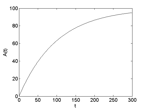
In the external influence model, the adoption coefficient only depends on an external factor. One such example in social media is when important news goes viral. Often, people who post or read the news don’t know each other; therefore, the importance of the news determines whether it goes viral. The external influence model can be formulated as
By solving Equation 7.28,
when A(t=t_0=0)=0. The A(t) function is shown in Figure 7.8. The number of adopters increases exponentially and then saturates near P.
Internal-Influence Model
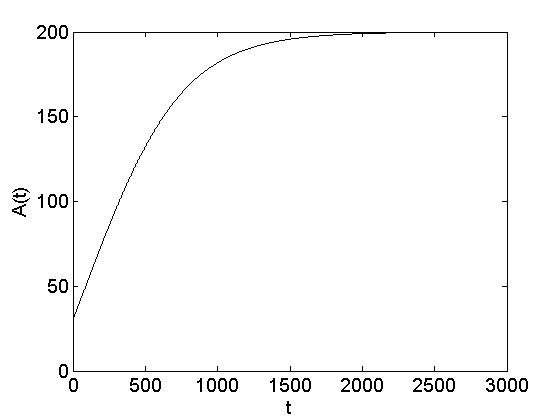
In the internal influence model, adoption depends on how many have adopted in the current timestep4. In social media this happens when a group of friends are joining a site due to peer pressure. Think of a group of individuals in a social networking site where the likelihood of joining increases as more group members join the site. The internal influence model can be described as follows:
Since the diffusion rate in this model depends on \beta A(t), it is called the pure imitation model
Pure Imitation Model. The solution to this model is defined as
where A(t=t_0) = A_0. The A(t) function is shown in Figure 7.9.
Mixed-Influence Model
As discussed, the mixed influence model is situated in between internal and external influence models. The mixed influence model is
By solving the differential equation, we arrive at
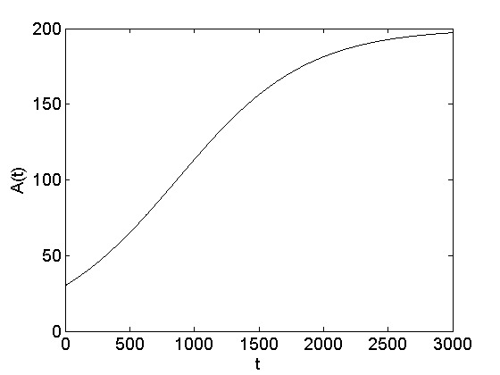
where A(t=t_0)=A_0. The A(t) function for the mixed influence model is depicted in Figure 7.10.
We discussed three models in this section: internal, external, and mixed influence. Depending on the model which is employed to describe the diffusion of innovations process, the respective equation for A(t) (Equations 7.29, 7.31, or 7.33) should be employed to model the system.
7.3.4 Intervention
Consider a faulty product being adopted. The product company is planning to stop or delay adoptions until the product is fixed and re-released. This intervention can performed by
Limiting the distribution of the product or the audience that can adopt the product. In our mathematical model, this is equivalent to reducing the population P that can potentially adopt the product.
Reducing interest in the product being sold. For instance, the company can inform adopters of the faulty status of the product. In our models, this can be achieved by tampering \alpha - setting \alpha to a very small value in 7.29 results in a slow adoption rate.
Reducing interactions within the population. Reduced interactions result in less imitations on product adoptions and a general decrease in the trend of adoptions. In our models, this can be achieved by setting \beta to a small value.
7.4 Epidemics
Epidemics describes the process by which diseases spread. This process consists of a pathogen (the disease being spread), a population of hosts (humans, animals, and plants, among others) and a spreading mechanism (breathing, drinking, sexual activity, etc.). Unlike information cascades and herding and similar to diffusion of innovations models, epidemic models assume an implicit network and unknown connections between individuals. This makes epidemic models more suitable when we are interested in global patterns, such as trends and ratios of people getting infected, and not in who infects whom.
In general, a complete understanding of the epidemic process requires substantial knowledge of the biological process within each host and the immune system process as well as a comprehensive analysis of interactions among individuals. Other factors such as social and cultural attributes also play a role in how, when, and where epidemics happen. Large epidemics, also known as pandemics, have spread through human populations, including the black death in the 13th century (killing more than 50% of Europe’s population), the Great plague of London (100,000 death toll), the Small pox, killing more than 90% of Massachusetts bay native Americans in the 17th century, and the recent ones, including HIV/AIDS, SARS, H5N1 (Avian flu), and influenza. These motivated the introduction of epidemic models in the early 20th century and the establishment of the epidemiology field.
There are various ways of modeling epidemics. For instance, one can look at how hosts contact each other and devise methods that describe how epidemics happen in networks. These networks are called contact networks
Contact Networks. A contact network is a graph where nodes represent the hosts and edges represent the interactions between these hosts. For instance, in the case of the HIV/AIDS, edges represent sexual interactions, and in the case of influenza, nodes that are connected represent hosts that breathe the same air. Nodes that are close in a contact network are not necessarily close in terms of real-world proximity. Real-world proximity might be true for plants or animals, but diseases such as SARS or avian flu travel between continents due to the traveling patterns of hosts. This becomes clearer when the science of epidemics is employed to understand the propagation of computer viruses in cell phone networks or across the Internet (Pastor-Satorras and Vespignani 2001; Newman et al. 2002).
Another way of looking at epidemic models is to avoid considering network information and analyze only the rates at which hosts get infected, recover, etc. This analysis is known as the fully-mixed
Fully-mixed
Techniquetechnique, assuming that each host han an equal chance of meeting others hosts. Through these interactions, hosts have random probabilities of getting infected. Though simplistic, the technique reveals several useful methods of modeling epidemics that are often capable of describing various real-world outbreaks. In this section, we concentrate on the fully-mixed models that avoid the use of contact networks 5.
Note that the fields that we discussed, such as diffusion of innovations or information cascades, are more or less related to epidemics. However, what makes epidemics different is that in the former, actors decide whether the innovation is adopted or the decision is taken and the system is usually fully observable. In epidemics, however, the system has a high level of uncertainty and the decisions of getting infected are not usually taken by individuals. The models discussed in this section assume that 1) no contact network information is available and 2) the process by which hosts get infected is unknown. These models can be applied to situations in social media where the decision process has a certain uncertainty to it or is ambiguous to the analyst.
7.4.1 Definitions
Since there is no network, we assume that we have a population where the disease is being spread. Let N define the size of this crowd. Any member of the crowd can be in either one of three states:
Susceptible: When an individual is in the susceptible state, he or she can potentially get infected by the disease. In reality, infections can come from outside the population where the disease is being spread (e.g., genetic mutation, an animal, etc.); however, for simplicity, we make a closed-world assumption, where susceptible individuals can only get infected by infected people in the population. We denote the number of susceptibles at time t as S(t) and the fraction of the population that is susceptible as s(t) = S(t)/N.
Infected: An infected individual has the chance of infecting susceptible parties. Let I(t) denote the number of infected individuals at time t and let i(t) denote the fraction of individuals that is infected, i(t) = I(t) / N.
Recovered (or Removed): These are individuals that are either recovered from the disease and hence have complete or partial immunity against the infection or killed by the infection. Let R(t) denotes the size of this set at time t and r(t) the fraction recovered, r(t)=R(t)/N .
Clearly, N = S(t) + I(t) + R(t) for all t. Since we are assuming that there is some level of randomness associated with the values of S(t), I(t), and R(t), we try to deal with expected values and assume S, I, and R represent these at time t.
7.4.2 SI Model
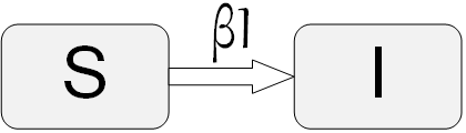
We start with the most basic model. In this model, the susceptible individuals get infected and once infected, they will never get cured. Denote \beta as the contact probability. In other words, the probability of a pair of people meeting in any time-step is \beta. So, if \beta=1, everyone comes into contact with everyone else, and if \beta=0, no one meets another individual. Assume that when an infected individual meets a susceptible individual the disease is being spread with probability 1 (this can be generalized to other values). Figure 7.11 demonstrates the SI model and the transition between states that happens in this model for individuals. The value over the arrow shows that each susceptible individual meets at least \beta I infected individuals during the next time-step.
Given this situation, infected individuals will meet \beta N people on average. We know from this set that only the fraction S/N will be susceptible and the rest are infected already. So, each infected individual will infect \beta NS/N = \beta S others. Since I individuals are infected, \beta IS will be infected in the next time-step. This means that the number of susceptible individuals will be reduced by this factor as well. So, to get different values of S and I at different times, we can solve the following differential equations:
Since S+I=N at all times, we can eliminate one equation by replacing S with N-I,
The solution to this differential equation is called the logistic growth function,
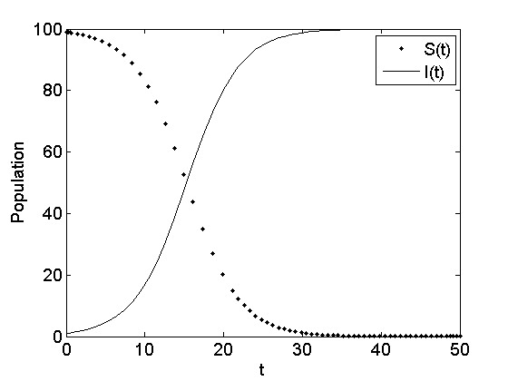
where I_0 is the number of individuals infected at time 0. In general, analyzing epidemics in terms of number of infected individuals has nominal generalization power. To address this, we can consider infected fractions. We therefore substitute i_0=\frac{I_0}{N} in the previous equation,
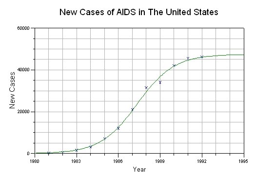
Note that in the limit, the SI model infects all the susceptible population since there is no recovery in the model. Figure 7.12(a) depicts the logistic growth function (infected individuals) and susceptible individuals for N=100, I_0=1, and \beta=0.003. Figure 7.12(b) depicts the infected population for HIV/AIDS for the past 20 years. As observed, the infected population can be approximated well with the logistic growth function and follows the SI model. Note that in the HIV/AIDS graph, not everyone is getting infected. This is because not everyone in the United States is in the susceptible population, so not everyone will get infected in the end. Moreover, there are other factors that are far more complex than the details of the SI model in how people get infected with HIV/AIDS.
7.4.3 SIR Model
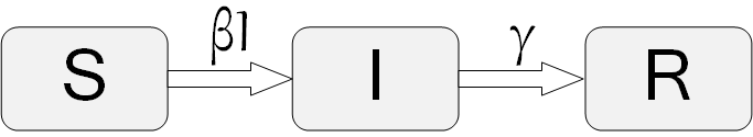
The SIR model, first introduced by Kermack and McKendrick (Kermack and McKendrick 1932), adds more detail to the standard SI model. In the SIR model, in addition to the I and S states, a recovery state R is present. Figure 7.13 depicts the model. In the SIR model, hosts get infected, remain infected for a while, and then recover. Once hosts recover (or are removed), they can no longer get infected and are no longer susceptible. The process by which susceptible individuals get infected is similar to the SI model, where a parameter \beta defines the probability of contacting others. Similarly, a parameter \gamma in the SIR model defines how infected people recover, or the recovering probability of an infected individual in a time period \Delta t.
In terms of differential equations, the SIR model is
Equation 7.39 is identical to that of the SI model (Equation 7.34). Equation 7.40 is different from Equation 7.35 of the SI model by the term \gamma I, which defines the number of infected individuals who recovered. These are removed from the infected set and are added to the recovered ones in Equation 7.41. Dividing Equation 7.41 by Equation 7.39, we get
and by assuming the number of recovered at time 0 is zero (R_0=0),
Since I+S+R=N, we replace I in Equation 7.41,
Now combining Equations 7.45 and 7.46,
If we solve this equation for R, then we can determine S from 7.45 and I from I=N-R-S. The solution for R can be computed by solving the following integration:
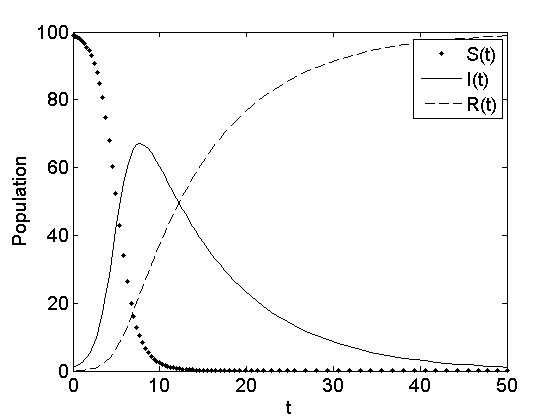
However, there is no closed form solution to this integration and only numerical approximation is possible. Figure 7.14 depicts the behavior of the SIR model for a set of initial parameters.
The two models in the next two subsections are generalized versions of the two models discussed thus far: SI and SIR. These models allow individuals to have temporary immunity and to get reinfected.
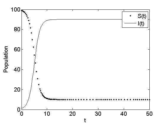
7.4.4 SIS Model
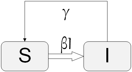
The SIS model is the same as the SI model, with the addition of infected nodes recovering and becoming susceptible again. The differential equations describing the model are
By replacing S with N-I in Eq. 7.50, we arrive at
When \beta N \le \gamma, the first term will be negative or zero at most; hence, the whole term becomes negative. Therefore, in the limit, the value I(t) will decrease exponentially to zero. However, when \beta N > \gamma, we will have a logistic growth function like the SI model. Having said this, as the simulation of the SIS model shows in Figure 7.16, the model will never infect everyone. It will reach a steady state, where both susceptibles and infecteds reach an equilibrium (see epidemic exercises) .
7.4.5 SIRS Model
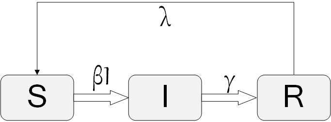
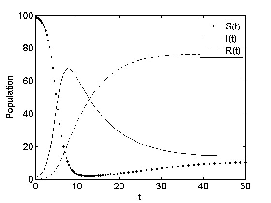
The final model analyzed in this section is the SIRS model. Similar to the SIS model, which extends the SI, the SIRS model will extend the SIR. The model is shown in Figure 7.17. In this model, the assumption is that individuals who have recovered will lose immunity after a certain period of time and will become susceptible again. A new parameter has been added to the model \lambda that defines the probability of losing immunity for a recovered individual. The set of differential equations that describes this model is
Like the SIR model, this model has no closed form solution, so numerical integration can be used. Figure 7.18 demonstrates a simulation of the SIRS model with given parameters of choice. As observed, the simulation outcome is similar to the SIR model simulation (see Figure 7.14). The major difference is that in the SIRS, number of susceptible and recovered individuals changes non-monotonically over time. For example, in SIRS, susceptible individuals decrease over time, but after reaching their minimum count, start increasing again. On the contrary, in the SIR, both susceptible individuals and recovered individuals change monotonically, where susceptible individuals decrease over time and recovered individuals increase over time. In both SIR and SIRS, the infected population changes non-monotonically.
7.4.6 Intervention
A pressing question in any pandemic or epidemic outbreak is how to stop the process. In this section, we discuss epidemic intervention based on a recent discovery by Nicholas A. Christakis (Christakis 2004). In any epidemic outbreak, infected individuals infect susceptible individuals. Although in this chapter we discuss random infection in the real world, what takes place is quite different. Infected individuals have a limited number of contacts and can only infect them if said contacts are susceptible. A well connected infected individual is more dangerous to the epidemic outbreak than someone who has no contacts. In other words, the epidemic takes place in a network. Unfortunately, it is often difficult to trace these contacts and outline their contact network. If this was possible, the best way to intervene with the epidemic outbreak would have been to vaccinate the highly connected nodes and stop the epidemic. This will result in what is known as the Herd Immunity and will stop the epidemic out-break. Herd immunity entails vaccinating a population inside a herd such that the pathogen cannot initiate an outbreak inside the herd. In general, creating herd immunity requires at least a random sample of 96% of the population to be vaccinated. Interestingly, we can achieve the same herd immunity by making use of friends in a network. In general, people know which of their friends have more friends. So, they know or have access to these higher degree and more connected nodes. Christakis found that if a random population of 30% of the herd is selected and then these 30% are asked for their highest-degree friends, by vaccinating these friends, one can achieve herd immunity. Of course, older intervention techniques such as separating the infecteds from the susceptibles (quarantining them) or removing the infecteds (killing cows with madcow disease) still work.
7.5 Summary
In this chapter, we discuss the concept of information diffusion in social networks. We first review the herding effect, where individuals observe the behaviors of others and act similarly to them based on their own benefit. We review the well-known diner example and urn experiment and demonstrate how conditional probabilities can be employed to discuss why herding takes place. We discuss how herding experiments should be designed and ways to intervene with it.
Next, we discuss the information cascade problem with the constraint of sequential decision making. The Independent Cascade Model (ICM) is discussed. The ICM is a sender-centric model and has a level of stochasticity associated with it. We discuss how the spread of cascades can be maximized in a network given a budget on how many initial nodes can be activated. Unfortunately, the problem is NP-Hard; therefore, we introduced a greedy approximation algorithm that has guaranteed performance due to the submodularity of ICM’s activation function. Finally, we discuss how to intervene with information cascades.
Our next topic is the diffusion of innovations. We discuss the characteristics of an adoption, both from the individual and innovation point of view. We reviewed well-known theories such as the models introduced by Ryan and Gross, Katz, and Rogers, in addition to experiments in the field, and different types of adopters. We also detailed mathematical models that account for internal, external, and mixed influences and their intervention procedures.
Finally, we move on to epidemics, an area where decision making is usually performed mindlessly. We discussed 4 different epidemic models: SI, SIR, SIS, and SIRS, where the two last models allow for reinfected individuals. Differential equations for each model are discussed, and numerical solutions as well as closed-form solutions, when available, were provided. We conclude the chapter with intervention approaches to epidemic outbreaks and a review of herd immunity in epidemics. We find that although a 96% random vaccination is required for achieving herd immunity, it is possible to achieve herd immunity by vaccinating a random population of 30% and vaccinating their highest-degree friends.
7.6 Bibliographic Notes
The concept of Herd has been well studied in psychology by Freud (Crowd Psychology), Carl Gustav Jung (Collective unconscious), and Gustave Le Bon (the popular mind). It has also been observed in economics by Veblen (Veblen 1965) and in studies related to the band-wagon effect (Rohlfs and Varian 2003; Simon 1954; Leibenstein 1950). The behavior is also discussed in terms of sociability (Simmel and Hughes 1949) in sociology.
Herding, first coined by Banerjee (Banerjee 1992), often refers to a slightly different concept. In herding, the crowd does not necessarily start with the same decision but will eventually reach one, whereas in herd behavior the same behavior is usually observed. Moreover, in herding, individuals decide whether the action they are taking has some benefits to themselves, and based on that, they will align with the population. In herd behavior, some level of uncertainty is associated with the decision and the individual doesn’t know why he or she is following the crowd.
Another confusion is that herd behavior/herding is often used interchangebly with information cascades (Bikhchandani et al. 1992; Welch 1992). To avoid this problem, we clearly define both in the chapter and assume that in herding decisions are taken based on global information, whereas in information cascades, local information is utilized.
Herd behavior has been studied in the context of financial markets (Cont and Bouchaud 2000; Drehmann et al. 2005; Bikhchandani and Sharma 2000; Devenow and Welch 1996) and investment (Scharfstein and Stein 1990). Gale analyzes the robustness of different herd models in terms of different constraints and externalities (Gale 1996) and Shiller discusses the relation between information, conversation, and herd behavior (Shiller 1995). Another well-known social conformity experiment has been conducted in Manhattan, NY by Milgram et al. (Milgram et al. 1969).
Other recent applications of threshold models can be found in (Young 2001; Watts 2002; Valente 1996a, 1995; Schelling 2006; Peleg 1997; Morris 2000; Macy and Willer 2002; Macy 1991; Granovetter 1978; Berger 2001). Bikhchandani et al. review conformity, fads, and information cascades in (Bikhchandani et al. 1998) and describe how observing past human decisions can help explain human behavior. Hirshleifer (Hirshleifer 1997) provides information cascade examples in many fields, including zoology, and finance, among others.
In terms of diffusion models, Robertson describes the process (Robertson 1967) and Hagerstrand (Hagerstrand et al. 1968) introduces a model based on the spatial stages of the diffusion of innovations and Montecarlo simulation models for diffusion of innovations. Bass (Bass 1969) discusses a model based on differential equations. Mahajan et al. (Mahajan and Peterson 1978) extend the Bass model.
Instances of external-influence models can be found in (Hamblin et al. 1973; Coleman et al. 1966) and internal-influence models are applied in (Mansfield 1961; Griliches 1957; Gray 1973). The Gompertz function (Martino 1993), widely used in forecasting, has direct relation with the internal-influence diffusion curve. Mixed-influence model examples include the work of Mahajan and Muller (Mahajan and Muller 1982) and Bass model (Bass 1969).
Midgley and Downling introduce the contingency model (Midgley and Dowling 1978). Abrahamson et al. mathematically analyze the bandwagon effect and diffusion of innovations. Their model predicts whether the bandwagon effect will occur and how many organizations will adopt the innovation. Network models of diffusion and thresholds for diffusion of innovations models are discussed by Valente (Valente 1996a, 1996b). Diffusion through blogspace and in general, social networks, has been analyzed by (Gruhl et al. 2004; Leskovec et al. 2007, n.d.; Yang and Leskovec 2010; Zafarani et al. 2010).
For information on different pandemics, refer to (Nohl et al. 1926; Bell et al. 1924; Patterson and Runge 2002; Des Jarlais et al. 1994; Dye and Gay 2003; Chinese et al. 2004, 2004; Guan et al. 2007; Nelson and Holmes 2007). To review some early and in-depth analysis of epidemic models, refer to (Bailey et al. 1975; Anderson and May 1992). Surveys of epidemics can be found in (Hethcote 2000, 1994; Hethcote et al. 1981; Dietz 1967). Epidemics in networks have been discussed (Newman 2010; Moore and Newman 2000; Keeling and Eames 2005) extensively. Other general sources include (Lewis 2009; Easley and Kleinberg 2010; Newman 2010; Barrat et al. 2008). A generalized model for contagion is provided by Watts et al. (Dodds and Watts 2004) and, in the case of best response dynamics, in (Morris 2000).
Other topics related to this chapter include wisdom of crowd models (Golub and Jackson 2010) and swarm intelligence (Eberhart et al. 2001; Poli et al. 2007; Engelbrecht 2005; Bonabeau et al. 1999; Kennedy 2006). One can also analyze information provenance, which aims to identify the sources from which information has diffused. Barbier et al. (Barbier et al. 2013) provide an overview of information provenance in social media in their book.
7.7 Exercises
Discuss how different information diffusion modeling techniques differ in nature. Name applications on social media that can make use of methods in each area.
Herd Effect
What are the minimum requirements for a herd behavior experiment? Design an experiment of your own.
Diffusion of Innovation
Simulate internal, external, and mixed influence models in a program. How are the saturation levels different for each model?
Provide a simple example of Diffusion of Innovations and suggest a specific way of intervention in order to expedite the diffusion.
Information Cascades
Briefly describe the Independent Cascade Model (ICM).
What is the objective of cascade maximization? What are the usual constraints?
Follow the ICM procedure until it converges for the following graph. Assume that node i activates node j when i-j \equiv 1~(mod~3) and node 1 is activated at time 0.
Epidemics
Discuss the mathematical relationship between the SIR and the SIS models.
Based on our assumptions in the SIR model , the probability that an individual remains infected follows a standard exponential distribution. Describe why this happens.
In the SIR model, what is the most likely time to recover based on the value of \gamma?
In the SIRS model, compute the length of time that an infected individual is likely to remain infected before they recover.
After the model saturates, how many are infected in the SIS model?
This assumption can be lifted (Kempe et al. 2003)↩︎
See (Gruhl et al. 2004) for an application in blogosphere.↩︎
Formally, assuming P\neq NP, there is no polynomial time algorithm for this problem.↩︎
The internal influence model is similar to the SI model discussed later on in epidemics. For the sake of completeness, we provide solutions to both in different sections. Readers are encouraged to refer to that model in Section 1.4 for further insight.↩︎
A generalization of these techniques over networks can be found in (Hethcote et al. 1981; Hethcote 1994; Newman 2010).↩︎