Graph Essentials
We live in a connected world in which networks are intertwined with our daily life. Networks of air and land transportation help us reach our destinations; critical infrastructure networks that distribute water and electricity are essential for our society and economy to function; and networks of communication help disseminate information at an unprecedented rate. Finally, our social interactions form social networks of friends, family, and colleagues. Social media attests to the growing body of these social networks in which individuals interact with one another through friendships, email, blogposts, buying similar products, and many other mechanisms.
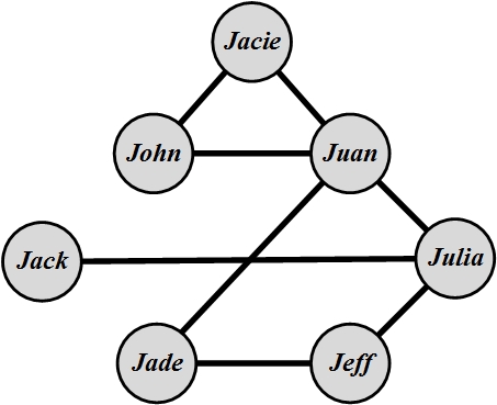
Social media mining aims to make sense of these individuals embedded in networks. These connected networks can be conveniently represented using graphs. As an example, consider a set of individuals on a social networking site where we want to find the most influential individual. Each individual can be represented using a node (circle) and two individuals who know each other can be connected with an edge (line). In Figure 2.1, we show a set of seven individuals and their friendships. Consider a hypothetical social theory that states that “the more individuals you know, the more influential you are.” This theory in our graph translates to the individual with the maximum degree (the number of edges connected to its corresponding node) being the most influential person. Therefore, in this network Juan is the most influential individual because he knows four others, which is more than anyone else. This simple scenario is an instance of many problems that arise in social media, which can be solved by modeling the problem as a graph. This chapter formally details the essentials required for using graphs and the fundamental algorithms required to explore these graphs in social media mining.
2.1 Graph Basics
In this section, we review some of the common notation used in graphs. Any graph contains both a set of objects, called nodes, and the connections between these nodes, called edges. Mathematically, a graph G is denoted as pair G(V,E), where V represents the set of nodes and E represents the set of edges. We formally define nodes and edges next.
2.1.1 Nodes
All graphs have fundamental building blocks. One major part of any graph is the set of nodes. In a graph representing friendship, these nodes represent people, and any pair of connected people denotes the friendship between them. Depending on the context, these nodes are called vertices or actors
Vertices and Actors. For example, in a web graph, nodes represent websites, and the connections between nodes indicate web-links between them. In a social setting, these nodes are called actors. The mathematical representation for a set of nodes is
where V is the set of nodes and v_i, 1 \le i \le n, is a single node. |V|=n is called the size of the graph. In Figure 2.1, n=7.
2.1.2 Edges
Another important element of any graph is the set of edges. Edges connect nodes. In a social setting, where nodes represent social entities such as people, edges indicate inter-node relationships and are therefore known as relationships or (social) ties
Relationships
and Ties. The edge set is usually represented using E,
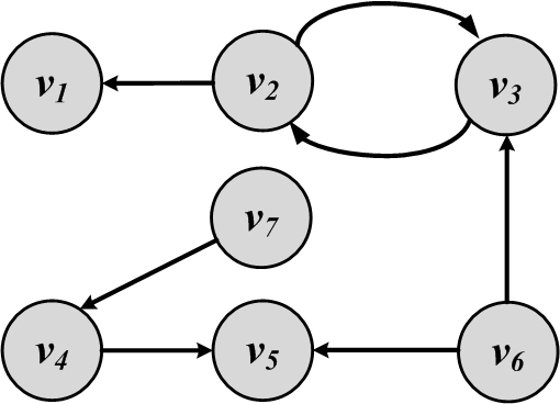
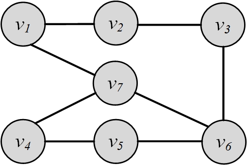
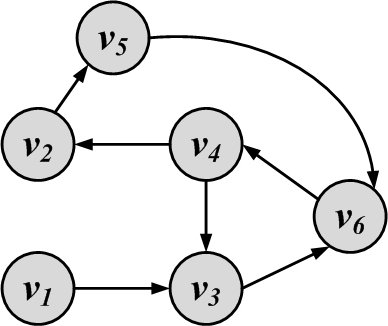
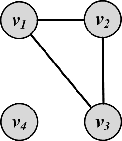
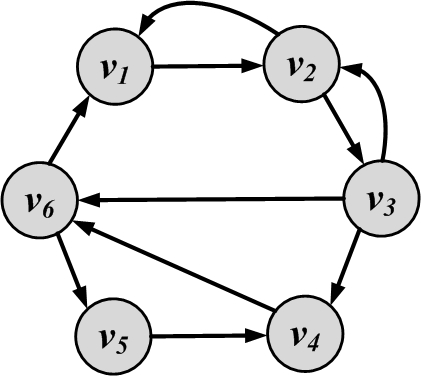
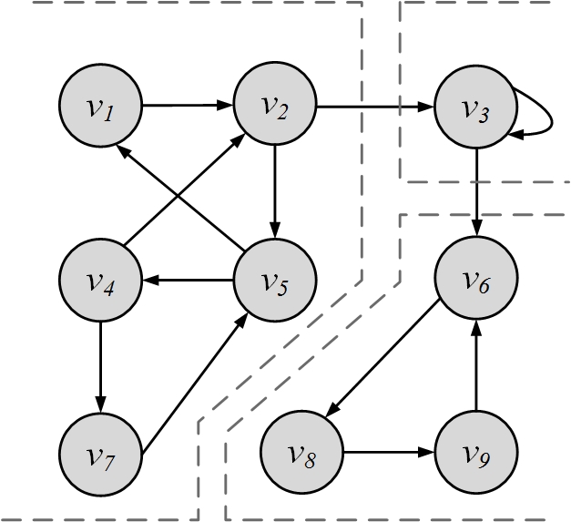
where e_i, 1 \le i \le m, is an edge and the size of the set is commonly shown as m=|E|. In Figure 2.1, lines connecting nodes represent the edges, so in this case, m=8. Edges are also represented by their endpoints (nodes), so e(v_1,v_2) (or (v_1,v_2)) defines an edge e between nodes v_1 and v_2. Edges can have directions, meaning one node is connected to another, but not vice versa. When edges are undirected, nodes are connected both ways. Note that in Figure 2.2(b), edges e(v_1,v_2) and e(v_2,v_1) are the same edges, because there is no direction in how nodes get connected. We call edges in this graph undirected edges and this kind of graph an undirected graph. Conversely, when edges have directions, e(v_1,v_2) is not the same as e(v_2,v_1). Graph 2.2(a) is a graph with directed edges; it is an example of a directed graph. Directed edges are represented using arrows. In a directed graph, an edge e(v_i,v_j) is represented using an arrow that starts at v_i and ends at v_j. Edges can start and end at the same node; these edges are called loops or self-links and are represented as e(v_i,v_i). For any node v_i, in an undirected graph, the set of nodes it is connected to via an edge is called its neighborhood
Neighborhoodand is represented as N(v_i). In Figure 2.1, N(Jade)=\{Jeff, Juan\}. In directed graphs, node v_i has incoming neighbors N_{\rm in}(v_i) (nodes that connect to v_i) and outgoing neighbors N_{\rm out}(v_i) (nodes that v_i connects to). In Figure 2.2(a), N_{\rm in}(v_2)=\{v_3\} and N_{\rm out}(v_2)=\{v_1,v_3\}.
2.1.3 Degree and Degree Distribution
The number of edges connected to one node is the degree of that node. Degree of a node v_i is often denoted using d_i. In the case of directed edges, nodes have in-degrees (edges pointing toward the node) and out-degrees (edges pointing away from the node). These values are presented using d_i^{\rm in} and d_i^{\rm out}, respectively. In social media, degree represents the number of friends a given user has. For example, on Facebook, degree represents the user’s number of friends, and on Twitter in-degree and out-degree represent the number of followers and followees, respectively. In any undirected graph, the summation of all node degrees is equal to twice the number of edges.
The summation of degrees in an undirected graph is twice the number of edges,
Proof. Any edge has two endpoints; therefore, when calculating the degrees d_i and d_j for any connected nodes v_i and v_j, the edge between them contributes 1 to both d_i and d_j; hence, if the edge is removed, d_i and d_j become d_i-1 and d_j-1, and the summation \sum_k d_k becomes \sum_k d_k - 2. Hence, by removal of all m edges, the degree summation becomes smaller by 2m. However, we know that when all edges are removed the degree summation becomes zero; therefore, the degree summation is 2\times m = 2|E|. ◻
In an undirected graph, there are an even number of nodes having odd degree.
Proof. The result can be derived from the previous theorem directly because the summation of degrees is even: 2|E|. Therefore, when nodes with even degree are removed from this summation, the summation of nodes with odd degree should also be even; hence, there must exist an even number of nodes with odd degree. ◻
In any directed graph, the summation of in-degrees is equal to the summation of out-degrees,
Proof. The proof is left as an exercise. ◻
Degree Distribution
In very large graphs, distribution of node degrees (degree distribution) is an important attribute to consider. The degree distribution plays an important role in describing the network being studied. Any distribution can be described by its members. In our case, these are the degrees of all nodes in the graph. The degree distribution p_d (or P(d), or P(d_v=d)) gives the probability that a randomly selected node v has degree d. Because p_d is a probability distribution \sum_{d=0}^{\infty}p_d=1. In a graph with n nodes, p_d is defined as
For the graph provided in Figure 2.1, the degree distribution p_d for d=\{1,2,3,4\} is
Because we have four nodes have degree 2, and degrees 1, 3, and 4 are observed once.
Power-law
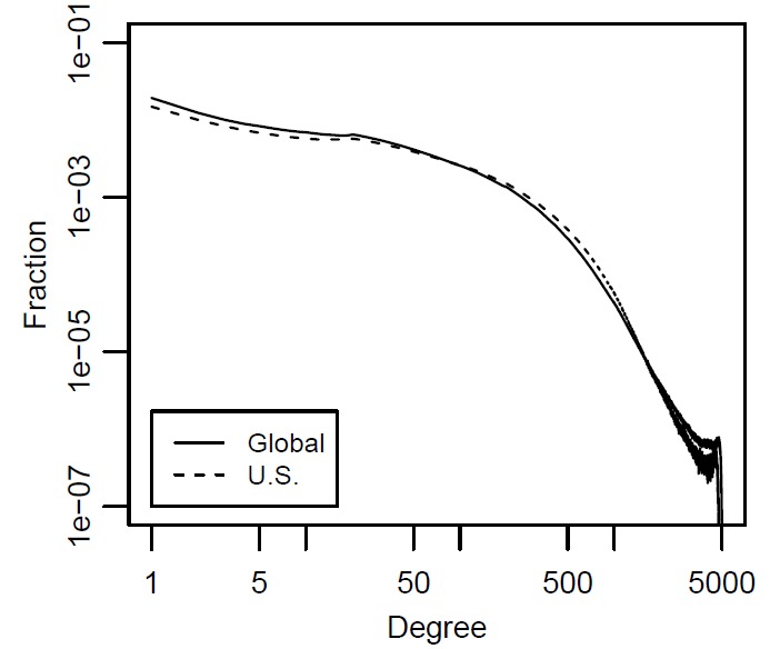
DistributionOn social networking sites, friendship relationships can be represented by a large graph. In this graph, nodes represent individuals and edges represent friendship relationships. We can compute the degrees and plot the degree distribution using a graph where the x-axis is the degree and the y-axis is the fraction of nodes with that degree.1 The degree distribution plot for Facebook in May 2012 is shown in Figure 2.3. A general trend observable on social networking sites is that there exist many users with few connections and there exist a handful of users with very large numbers of friends. This is commonly called the power-law degree distribution.
As previously discussed, any graph G can be represented as a pair G(V,E), where V is the node set and E is the edge set. Since edges are between nodes, we have
Graphs can also have subgraphs. For any graph G(V,E), a graph G'(V',E') is a subgraph of G(V,E), if the following properties hold:
2.2 Graph Representation
We have demonstrated the visual representation of graphs. This representation, although clear to humans, cannot be used effectively by computers or manipulated using mathematical tools. We therefore seek representations that can store the node and edge sets in a way that (1) does not lose information, (2) can be manipulated easily by computers, and (3) can have mathematical methods applied easily.
Adjacency Matrix
A simple way of representing graphs is to use an adjacency matrix (also known as a sociomatrix)
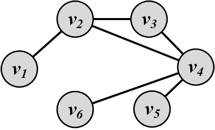
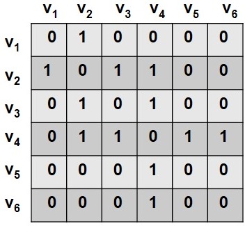
Sociomatrix. Figure 2.4 depicts an example of a graph and its corresponding adjacency matrix. A value of 1 in the adjacency matrix indicates a connection between nodes v_i and v_j, and a 0 denotes no connection between the two nodes. When generalized, any real number can be used to show the strength of connections between two nodes. The adjacency matrix gives a natural mathematical representation for graphs. Note that in social networks, because of the relatively small number of interactions, many cells remain zero. This creates a large sparse matrix. In numerical analysis, a sparse matrix is one that is populated primarily with zeros.
In the adjacency matrix, diagonal entries represent self-links or loops. Adjacency matrices can be commonly formalized as
Adjacency List
In an adjacency list, every node is linked with a list of all the nodes that are connected to it. The list is often sorted based on node order or some other preference. For the graph shown in Figure 2.4, the corresponding adjacency list is shown in Table 1.1.
| Node | Connected To |
|---|---|
| v_1 | v_2 |
| v_2 | v_1,v_3,v_4 |
| v_3 | v_2,v_4 |
| v_4 | v_2,v_3,v_5,v_6 |
| v_5 | v_4 |
| v_6 | v_4 |
Edge List
Another simple and common approach to storing large graphs is to save all edges in the graph. This is known as the edge list representation. For the graph shown in Figure 2.4, we have the following edge list representation:
In this representation, each element is an edge and is represented as (v_i,v_j), denoting that node v_i is connected to node v_j. Since social media networks are sparse, both the adjacency list and edge list representations save significant space. This is because many zeros need to be stored when using adjacency matrices, but do not need to be stored in an adjacency or an edge list.
2.3 Types of Graphs
In general, there are many basic types of graphs. In this section we discuss several basic types of graphs.
Null Graph. A null graph is a graph where the node set is empty (there are no nodes). Obviously, since there are no nodes, there are also no edges. Formally,
Empty Graph. An empty or edgeless graph is one where the edge set is empty:
Note that the node set can be non-empty. A null graph is an empty graph but not vice versa.
Directed/Undirected/Mixed Graphs. Graphs that we have discussed thus far rarely had directed edges. As mentioned, graphs that only have directed edges are called directed graphs and ones that only have undirected ones are called undirected graphs. Mixed graphs have both directed and undirected edges. In directed graphs, we can have two edges between i and j (one from i to j and one from j to i), whereas in undirected graphs only one edge can exist. As a result, the adjacency matrix for directed graphs is not in general symmetric (i connected to j does not mean j is connected to i, i.e., A_{i,j} \neq A_{j,i}), whereas the adjacency matrix for undirected graphs is symmetric (A=A^T).
In social media, there are many directed and undirected networks. For instance, Facebook is an undirected network in which if Jon is a friend of Mary, then Mary is also a friend of Jon. Twitter is a directed network, where follower relationships are not bidirectional. One direction is called followers, and the other is denoted as following.
Simple Graphs and Multigraphs. In the example graphs that we have provided thus far, only one edge could exist between any pair of nodes. These graphs are denoted as simple graphs. Multigraphs are graphs where multiple edges between two nodes can exist. The adjacency matrix for multigraphs can include numbers larger than one, indicating multiple edges between nodes. Multigraphs are frequently observed in social media where two individuals can have different interactions with one another. They can be friends and, at the same time, colleagues, group members, or other relation. For each one of these relationships, a new edge can be added between the individuals, creating a multigraph.
Weighted Graphs. A weighted graph is one in which edges are associated with weights. For example, a graph could represent a map, where nodes are cities and edges are routes between them. The weight associated with each edge represents the distance between these cities. Formally, a weighted graph can be represented as G(V,E,W), where W represents the weights associated with each edge, |W|=|E|. For an adjacency matrix representation, instead of 1/0 values, we can use the weight associated with the edge. This saves space by combining E and W into one adjacency matrix A, assuming that an edge exists between v_i and v_j if and only if W_{ij} \neq 0. Depending on the context, this weight can also be represented by w_{ij} or w(i,j).
An example of a weighted graph is the web graph. A web graph is a way of representing how internet sites are connected on the web. In general, a web graph is a directed graph. Nodes represent sites and edge weights represent number of links between sites. Two sites can have multiple links pointing to each other, and individual sites can have loops (links pointing to themselves).
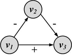
A special case of a weighted graph is when we have binary weights (0/1 or +/-) on edges. These edges are commonly called signed edges, and the weighted graph is called a signed graph
Signed Edges and
Signed Graphs. Signed edges can be employed to represent contradictory behavior. For instance, one can use signed edges to represent friends and foes. A positive (+) edge between two nodes represents friendship, and a negative (-) edge denotes that the endpoint nodes (individuals) are considered enemies. When edges are directed, one endpoint considers the other endpoint a friend or a foe, but not vice versa. When edges are undirected, endpoints are mutually friends or foes. In another setting, a + edge can denote a higher social status, and a - edge can represent lower social status. Social status is the rank assigned to one’s position in society. For instance, a school principal can be connected via a directed + edge to a student of the school because, in the school environment, the principal is considered to be of higher status. Figure 2.5 shows a signed graph consisting of nodes and the signed edges between them.
2.4 Connectivity in Graphs
Connectivity defines how nodes are connected via a sequence of edges in a graph. Before we define connectivity, some preliminary concepts need to be detailed.
Adjacent Nodes and Incident Edges. Two nodes v_1 and v_2 in graph G(V,E) are adjacent when v_1 and v_2 are connected via an edge:
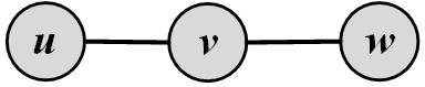
Two edges e_1(a,b) and e_2(c,d) are incident when they share one endpoint (i.e., are connected via a node):
Figure 2.6 depicts adjacent nodes and incident edges in a sample graph. In a directed graph, two edges are incident if the ending of one is the beginning of the other; that is, the edge directions must match for edges to be incident.
Traversing an Edge. An edge in a graph can be traversed when one starts at one of its end-nodes, moves along the edge, and stops at its other end-node. So, if an edge e(a,b) connects nodes a and b, then visiting e can start at a and end at b. Alternatively, in an undirected graph we can start at b and end the visit at a.
Walk, Path, Trail, Tour, and Cycle. A walk is a sequence of incident edges traversed one after another. In other words, if in a walk one traverses edges e_1(v_1,v_2),e_2(v_2,v_3),e_3(v_3,v_4),\dots,e_n(v_n,v_{n+1}), we have v_1 as the walk’s starting node and v_{n+1} as the walk’s ending node. When a walk does not end where it started (v_1 \neq v_{n+1}) then it is called an open walk. When
Open Walk and
Closed Walka walk returns to where it was started (v_1 = v_{n+1}), it is called a closed walk. Similarly, a walk can be denoted as a sequence of nodes, v_1, v_2, v_3, \dots, v_n. In this representation, the edges that are traversed are e_1(v_1,v_2), e_2(v_2,v_3), \dots, e_{n-1}(v_{n-1},v_n). The length of a walk is the number of edges traversed during the walk and in our case is n-1.
A trail is a walk where no edge is traversed more than once; therefore, all walk edges are distinct. A closed trail (one that ends where it started) is called a tour or circuit.
A walk where nodes and edges are distinct is called a path, and a closed path is called a cycle. The length of a path or cycle is the number of edges traversed in the path or cycle. In a directed graph, we have directed paths because traversal of edges is only allowed in the direction of the edges. In Figure 2.7, v_4,v_3,v_6,v_4,v_2 is a walk; v_4,v_3 is a path; v_4, v_3, v_6, v_4, v_2 is a trail; and v_4, v_3, v_6, v_4 is both a tour and a cycle.
A graph has a Hamiltonian cycle if it has a cycle such that all the nodes in the graph are visited. It has an Eulerian tour if all the edges are traversed only once. Examples of a Hamiltonian cycle and an Eulerian tour are provided in Figure 2.8.
One can perform a random walk on a weighted graph
Random Walk, where nodes are visited randomly. The weight of an edge, in this case, defines the probability of traversing it. For this to work correctly, we must make sure that for all edges that start at v_i we have
The random walk procedure is outlined in Algorithm 2.1. The algorithm starts at a node v_0 and visits its adjacent nodes based on the transition probability (weight) assigned to edges connecting them. This procedure is performed for t steps (provided to the algorithm); therefore, a walk of length t is generated by the random walk.
- Require: Initial Node v_0, Weighted Graph G(V,E,W), Steps t
- return Random Walk P
- state = 0;
- v_t = v_0;
- P=\{v_0\};
- while state < t do
- state = state + 1;
- select a random node v_j adjacent to v_t with probability w_{t,j};
- v_t=v_j;
- P=P \cup \{v_j\};
- end while
- Return P
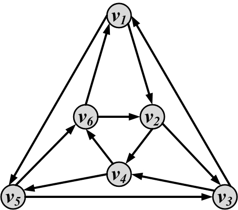
Connectivity. A node v_i is connected to node v_j (or v_j is reachable from v_i) if it is adjacent to it or there exists a path from v_i to v_j. A graph is connected if there exists a path between any pair of nodes in it. In a directed graph, the graph is weakly connected if there exists a path between any pair of nodes, without following the edge directions (i.e., directed edges are replaced with undirected edges). The graph is strongly connected if there exists a directed path (following edge directions) between any pair of nodes. Figure 2.9 shows examples of connected, disconnected, weakly connected, and strongly connected graphs.
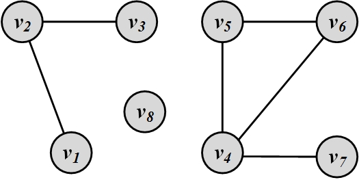
Components. A component in an undirected graph is a subgraph such that, there exists a path between every pair of nodes inside the component. Figure 2.10(b)(a) depicts an undirected graph with three components. A component in a directed graph is strongly connected if, for every pair of nodes v and u, there exists a directed path from v to u and one from u to v. The component is weakly connected if replacing directed edges with undirected edges results in a connected component. A graph with three strongly connected components is shown in Figure 2.10(b)(b).
Shortest Path. When a graph is connected, multiple paths can exist between any pair of nodes. Often, we are interested in the path that has the shortest length. This path is called the shortest path. Applications for shortest paths include GPS routing, where users are interested in the shortest path to their destination. In this chapter, we denote the length of the shortest path between nodes v_i and v_j as l_{i,j}. The concept of the neighborhood of a node v_i can be generalized using shortest paths. An n-hop neighborhood of node v_i is the set of nodes that are within n hops distance from node v_i. That is, their shortest path to v_i has length less than or equal to n.
Diameter. The diameter of a graph is defined as the length of the longest shortest path between any pair of nodes in the graph. It is defined only for connected graphs because the shortest path might not exist in disconnected graphs. Formally, for a graph G, the diameter is defined as
2.5 Special Graphs
Using general concepts defined thus far, many special graphs can be defined. These special graphs can be used to model different problems. We review some well-known special graphs and their properties in this section.
2.5.1 Trees and Forests
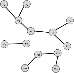
Trees are special cases of undirected graphs. A tree is a graph structure that has no cycle in it. In a tree, there is exactly one path between any pair of nodes. A graph consisting of set of disconnected trees is called a forest. A forest is shown in Figure 2.11.
In a tree with |V| nodes, we have |E|=|V|-1 edges. This can be proved by contradiction (see Exercises).
2.5.2 Special Subgraphs
Some subgraphs are frequently used because of their properties. Two such subgraphs are discussed here.
Spanning Tree. For any connected graph, the spanning tree is a subgraph and a tree that includes all the nodes of the graph. Obviously, when the original graph is not a tree, then its spanning tree includes all the nodes, but not all the edges. There may exist multiple spanning trees for a graph. For a weighted graph and one of its spanning trees, the weight of that spanning tree is the summation of the edge weights in the tree. Among the many spanning trees found for a weighted graph, the one with the minimum weight is called the minimum spanning tree (MST) .
For example, consider a set of cities, where roads need to be built to connect them. We know the distance between each pair of cities. We can represent each city with a node and the distance between these nodes using an edge between them labeled with the distance. This graph-based view is shown in Figure 2.12. In this graph, nodes v_1, v_2, …, v_9 represent cities, and the values attached to edges represent the distance between them. Note that edges only represent distances (potential roads!), and roads may not exist between these cities. Due to construction costs, the government needs to minimize the total mileage of roads built and, at the same time, needs to guarantee that there is a path (i.e., a set of roads) that connects every two cities. The minimum spanning tree is a solution to this problem. The edges in the MST represent roads that need to be built to connect all of the cities at the minimum length possible. Figure 2.2 highlights the minimum spanning tree.
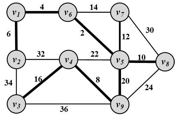
Figure 2.12: Minimum Spanning Tree. Nodes represent cities and values assigned to edges represent geographical distance between cities. Highlighted edges are roads that are built in a way that minimizes their total length. Steiner Tree. The Steiner Tree problem is similar to the minimum spanning tree problem. Given a weighted graph G(V,E,W) and a subset of nodes V' \subseteq V (terminal nodes
Terminal nodes) , the Steiner tree problem aims to find a tree such that it spans all the V' nodes and the weight of the tree is minimized. Note that the problem is different from the MST problem because we do not need to span all nodes of the graph V, but only a subset of the nodes V'. A Steiner tree example is shown in Figure 2.13. In this example, V'=\{v_2,v_4,v_7\}.
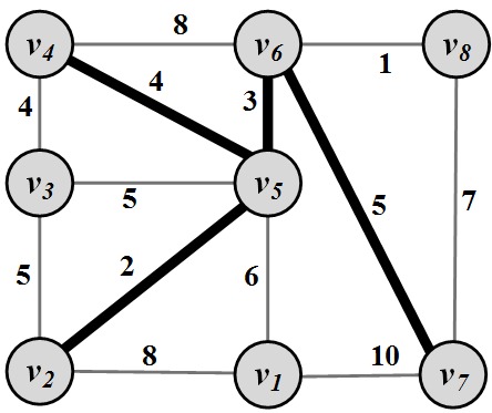
Figure 2.13: Steiner tree for V'=\{v_2,v_4,v_7\}.
2.5.3 Complete Graphs
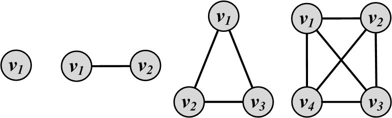
A complete graph is a graph where for a set of nodes V, all possible edges exist in the graph. In other words, all pairs of nodes are connected with an edge. Hence,
Complete graphs with n nodes are often denoted as K_n. K_1, K_2, K_3, and K_4 are shown in Figure 2.14.
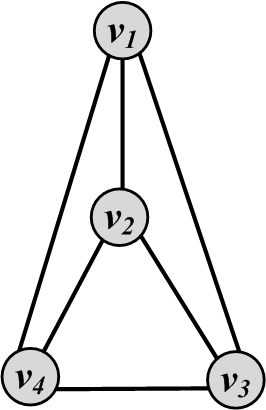
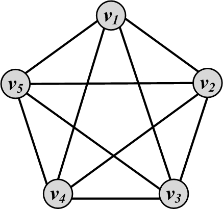
2.5.4 Planar Graphs
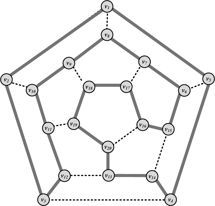
A graph that can be drawn in such a way that no two edges cross each other (other than the endpoints) is called planar. A graph that is not planar is denoted as nonplanar. Figure 2.15 shows an example of a planar graph and a nonplanar graph.
2.5.5 Bipartite Graphs
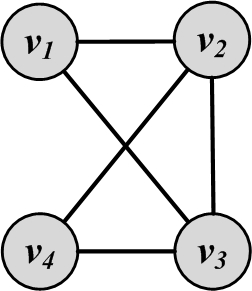
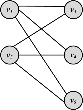
A bipartite graph G(V,E) is a graph where the node set can be partitioned into two sets such that, for all edges, one endpoint is in one set and the other endpoint is in the other set. In other words, edges connect nodes in these two sets, but there exist no edges between nodes that belong to the same set. Formally,
Figure 2.16(a) shows a sample bipartite graph. In this figure, V_L=\{v_1,v_2\} and V_R=\{v_3,v_4,v_5\}.
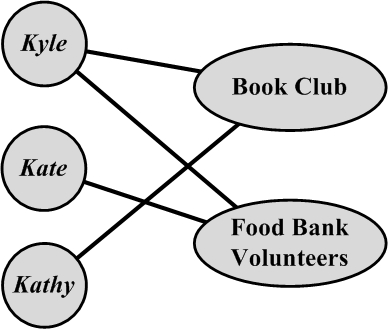
In social media, affiliation networks are well-known examples of bipartite graphs. In these networks, nodes in one part (V_L or V_R) represent individuals, and nodes in the other part represent affiliations. If an individual is associated with an affiliation, an edge connects the corresponding nodes. A sample affiliation network is shown in Figure 2.16(b).
2.5.6 Regular Graphs
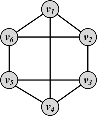
A regular graph is one in which all nodes have the same degree. A regular graph where all nodes have degree 2 is called a 2-regular graph. More generally, a graph where all nodes have degree k is called a k-regular graph. Regular graphs can be connected or disconnected. Complete graphs are examples of regular graphs, where all n nodes have degree n-1 (i.e., k=n-1). Cycles are also regular graphs, where k=2. Another example for k=3 is shown in Figure 2.17.
2.5.7 Bridges
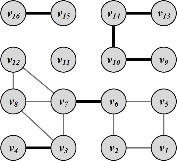
Consider a graph with several connected components. Edges in this graph whose removal will increase the number of connected components are called bridges. As the name suggests, these edges act as bridges between connected components. The removal of these edges results in the disconnection of formerly connected components and hence an increase in the number of components. An example graph and all its bridges are depicted in Figure 2.18.
2.6 Graph Algorithms
In this section, we review some well-known algorithms for graphs, although they are only a small fraction of the plethora of algorithms related to graphs.
2.6.1 Graph/Tree Traversal
Among the most useful algorithms for graphs are the traversal algorithms for graphs, and special subgraphs, such as trees. Consider a social media site that has many users, and we are interested in surveying it and computing the average age of its users. The usual technique is to start from one user and employ some traversal technique to browse his friends and then these friends’ friends and so on. The traversal technique guarantees that (1) all users are visited and (2) no user is visited more than once.
In this section, we discuss two traversal algorithms: depth-first search (DFS) and breadth-first search (BFS).
Depth-First Search (DFS)
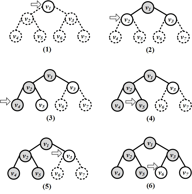
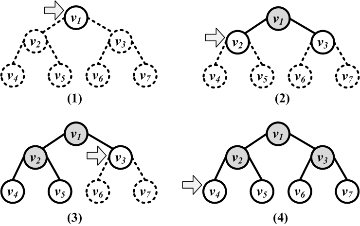
Depth-first search (DFS) starts from a node v_i, selects one of its neighbors v_j \in N(v_i), and performs DFS on v_j before visiting other neighbors in N(v_i). In other words, DFS explores as deep as possible in the graph using one neighbor before backtracking to other neighbors. Consider a node v_i that has neighbors v_j and v_k; that is, v_j, v_k \in N(v_i). Let v_{j(1)} \in N(v_j) and v_{j(2)} \in N(v_j) denote neighbors of v_j such that v_i \neq v_{j(1)} \neq v_{j(2)}. Then for a depth-first search starting at v_i, that visits v_j next, nodes v_{j(1)} and v_{j(2)} are visited before visiting v_k. In other words, a deeper node v_{j(1)} is preferred to a neighbor v_k that is closer to v_i. Depth-first search can be used both for trees and graphs, but is better visualized using trees. The DFS execution on a tree is shown in Figure 2.19(a).
The DFS algorithm is provided in Algorithm 2.2. The algorithm uses a stack structure to visit nonvisited nodes in a depth-first fashion.
- Require: Initial node v, graph/tree G(V,E), stack S
- return An ordering on how nodes in G are visited
- Push v into S;
- visitOrder = 0;
- while S not empty do
- node = pop from S;
- if node not visited then
- visitOrder = visitOrder +1;
- Mark node as visited with order visitOrder;
//or print node - Push all neighbors/children of node into S;
- end if
- end while
- Return all nodes with their visit order.
Breadth-First Search (BFS)
Breadth-first search (BFS) starts from a node, visits all its immediate neighbors first, and then moves to the second level by traversing their neighbors. Like DFS, the algorithm can be used both for trees and graphs and is provided in Algorithm 2.3.
The algorithm uses a queue data structure to achieve its goal of breadth traversal. Its execution on a tree is shown in Figure 2.19(b).
In social media, we can use BFS or DFS to traverse a social network: the algorithm choice depends on which nodes we are interested in visiting first. In social media, immediate neighbors (i.e., friends) are often more important to visit first; therefore, it is more common to use breadth-first search.
- Require: Initial node v, graph/tree G(V,E), queue Q
- return An ordering on how nodes are visited
- Enqueue v into queue Q;
- visitOrder = 0;
- while Q not empty do
- node = dequeue from Q;
- if node not visited then
- visitOrder = visitOrder +1;
- Mark node as visited with order visitOrder;
//or print node - Enqueue all neighbors/children of node into Q;
- end if
- end while
2.6.2 Shortest Path Algorithms
In many scenarios, we require algorithms that can compute the shortest path between two nodes in a graph. For instance, in the case of navigation, we have a weighted network of cities connected via roads, and we are interested in computing the shortest path from a source city to a destination city. In social media mining, we might be interested in determining how tightly connected a social network is by measuring its diameter. The diameter can be calculated by finding the longest shortest path between any two nodes in the graph.
Dijkstra’s Algorithm
A well-established shortest path algorithm was developed in 1959 by Edsgerd Dijkstra. The algorithm is designed for weighted graphs with non-negative edges. The algorithm finds the shortest paths that start from a starting node s to all other nodes and the lengths of those paths.
- Require: Start node s, weighted graph/tree G(V,E,W)
- return Shortest paths and distances from s to all other nodes.
- for v \in V do
- distance[v] = \infty;
- predecessor[v] = -1;
- end for
- distance[s] = 0;
- unvisited = V;
- while unvisited \neq \emptyset do
- smallest = {arg\,min}_{v \in unvisited} distance(v);
- if distance(smallest){=}{=} \infty then
- break;
- end if
- unvisited = unvisited \setminus \{smallest\};
- currentDistance = distance(smallest);
- for adjacent node to smallest: neighbor \in unvisited do
- newPath = currentDistance{+}w(smallest, neighbor);
- if newPath < distance(neighbor) then
- distance(neighbor)=newPath;
- predecessor(neighbor)=smallest;
- end if
- end for
- end while
- Return distance[] and predecessor[] arrays
The Dijkstra’s algorithm is provided in Algorithm 2.4. As mentioned, the goal is to find the shortest paths and their lengths from a source node s to all other nodes in the graph. The distance array (Line 3) keeps track of the shortest path distance from s to other nodes. The algorithm starts by assuming that there is a shortest path of infinite length to any node, except s, and will update these distances as soon as a better distance (shorter path) is observed. The steps of the algorithm are as follows:
All nodes are initially unvisited. From the unvisited set of nodes, the one that has the minimum shortest path length is selected. We denote this node as smallest in the algorithm.
For this node, we check all its neighbors that are still unvisited. For each unvisited neighbor, we check if its current distance can be improved by considering the shortest path that goes through smallest. This can be performed by comparing its current shortest path length (distance(neighbor)) to the path length that goes through smallest (distance(smallest){+}w(smallest, neighbor)). This condition is checked in Line 17.
If the current shortest path can be improved, the path and its length are updated. The paths are saved based on predecessors in the path sequence. Since, for every node, we only need the predecessor to reconstruct a path recursively, the predecessor array keeps track of this.
A node is marked as visited after all its neighbors are processed and is no longer changed in terms of (1) the shortest path that ends with it and (2) its shortest path length.
To further clarify the process, an example of the Dijkstra’s algorithm is provided.
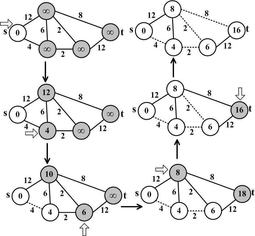
Figure 2.20 provides an example of the Dijkstra’s shortest path algorithm. We are interested in finding the shortest path between s and t. The shortest path is highlighted using dashed lines. In practice, shortest paths are saved using the predecessor array.
- Require: Connected weighted graph G(V,E,W)
- return Spanning tree T(V_s,E_s)
- V_s = {a random node from V};
- E_s = {};
- while V \neq V_s do
- e(u,v) = argmin_{(u,v),u \in V_s, v \in V-V_s} w(u,v)
- V_s = V_s \cup \{v\};
- E_s = E_s \cup e(u,v);
- end while
- Return tree T(V_s, E_s) as the minimum spanning tree;
2.6.3 Minimum Spanning Trees
A spanning tree of a connected undirected graph is a tree that includes all the nodes in the original graph and a subset of its edges. Spanning trees play important roles in many real-life applications. A cable company that wants to lay wires wishes not only to cover all areas (nodes) but also minimize the cost of wiring (summation of edges). In social media mining, consider a network of individuals who need to be provided with a piece of information. The information spreads via friends, and there is a cost associated with spreading information among every two nodes. The minimum spanning tree of this network will provide the minimum cost required to inform all individuals in this network.
There exist a variety of algorithms for finding minimum spanning trees. A famous algorithm for finding MSTs in a weighted graph is Prim’s algorithm (Prim 1957). Interested readers can refer to the bibliographic notes for further references.
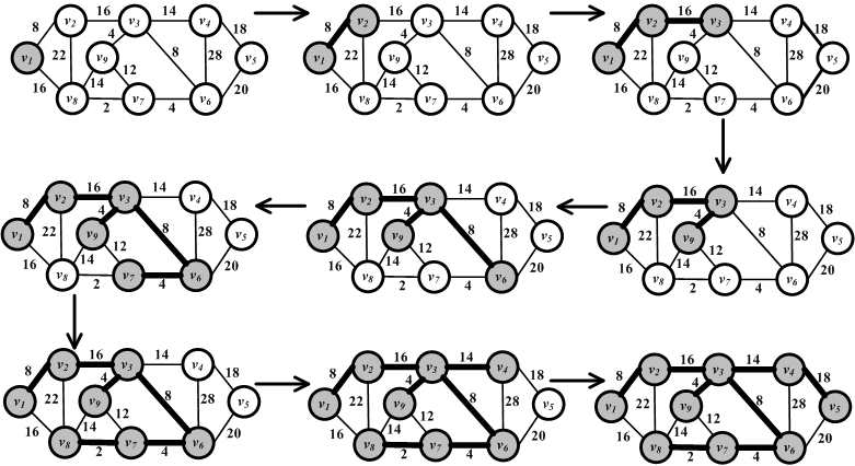
Prim’s Algorithm
Prim’s algorithm is provided in Algorithm 2.5. It starts by selecting a random node and adding it to the spanning tree. It then grows the spanning tree by selecting edges that have one endpoint in the existing spanning tree and one endpoint among the nodes that are not selected yet. Among the possible edges, the one with the minimum weight is added to the set (along with its endpoint). This process is iterated until the graph is fully spanned. An example of Prim’s algorithm is provided in Figure 2.21.
2.6.4 Network Flow Algorithms
Consider a network of pipes that connect an infinite water source to a water sink. In these networks, given the capacity of these pipes, an interesting question is, What is the maximum flow that can be sent from the source to the sink?
Network flow algorithms aim to answer this question. This type of question arises in many different fields. At first glance, these problems do not seem to be related to network flow algorithms, but there are strong parallels. For instance, in social media sites where users have daily limits (the capacity, here) of sending messages (the flow) to others, what is the maximum number of messages the network should be prepared to handle at any time?
Before we delve into the details, let us formally define a flow network.
Flow Network
A flow network G(V,E,C)2 is a directed weighted graph, where we have the following:
\forall~e(u,v) \in E, c(u,v) \ge 0 defines the edge capacity.
When (u,v) \in E, (v,u) \not \in E (opposite flow is impossible).
s defines the source node
Source and Sinkand t defines the sink node. An infinite supply of flow is connected to the source.
A sample flow network, along with its capacities, is shown in Figure 2.22.
Flow
Given edges with certain capacities, we can fill these edges with the flow up to their capacities. This is known as the capacity constraint. Furthermore, we should guarantee that the flow that enters any node other than source s and sink t is equal to the flow that exits it so that no flow is lost (flow conservation constraint). Formally,
\forall (u,v) \in E, f(u,v) \ge 0 defines the flow passing through that edge.
\forall (u,v) \in E, 0 \le f(u,v) \le c(u,v) (capacity constraint).
\forall v \in V, v \not \in \{s,t\}, \sum_{k: (k,v) \in E} f(k,v) = \sum_{l: (v,l) \in E} f(v,l) (flow conservation constraint).
Commonly, to visualize an edge with capacity c and flow f, we use the notation f/c. A sample flow network with its flows and capacities is shown in Figure 2.23.
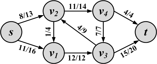
Flow Quantity
The flow quantity (or value of the flow) in any network is the amount of outgoing flow from the source minus the incoming flow to the source. Alternatively, one can compute this value by subtracting the outgoing flow from the sink from its incoming value:
The flow quantity for the example in Figure 2.23 is 19:
Our goal is to find the flow assignments to each edge with the maximum flow quantity. This can be achieved by a maximum flow algorithm. A well-established one is the Ford-Fulkerson algorithm (Ford and Fulkerson 1956).
Ford-Fulkerson Algorithm
The intuition behind this algorithm is as follows: Find a path from source to sink such that there is unused capacity for all edges in the path. Use that capacity (the minimum capacity unused among all edges on the path) to increase the flow. Iterate until no other path is available.
Before we formalize this, let us define some concepts.
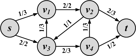
Given a flow in network G(V,E,C), we define another network G_R(V, E_R, C_R), called the residual network. This network defines how much capacity remains in the original network. The residual network has an edge between nodes u and v if and only if either (u,v) or (v,u) exists in the original graph. If one of these two exists in the original network, we would have two edges in the residual network: one from (u,v) and one from (v,u). The intuition is that when there is no flow going through an edge in the original network, a flow of as much as the capacity of the edge remains in the residual. However, in the residual network, one has the ability to send flow in the opposite direction to cancel some amount of flow in the original network.
The residual capacity c_R(u,v) for any edge (u,v) in the residual graph is
A flow network example and its resulted residual network are shown in Figure 2.24. In the residual network, edges that have zero residual capacity are not shown.
Augmentation and Augmenting Paths
In the residual graph, when edges are in the same direction as the original graph, their capacity shows how much more flow can be pushed along that edge in the original graph. When edges are in the opposite direction, their capacities show how much flow can be pushed back on the original graph edge. So, by finding a flow in the residual, we can augment the flow in the original graph. Any simple path from s to t in the residual graph is an augmenting path. Since all capacities in the residual are positive, these paths can augment flows in the original, thus increasing the flow. The amount of flow that can be pushed along this path is equal to the minimum capacity along the path, since the edge with that capacity limits the amount of flow being pushed.3
Weak linkGiven flow f(u,v) in the original graph and flow f_R(u,v) and f_R(v,u) in the residual graph, we can augment the flow as follows:
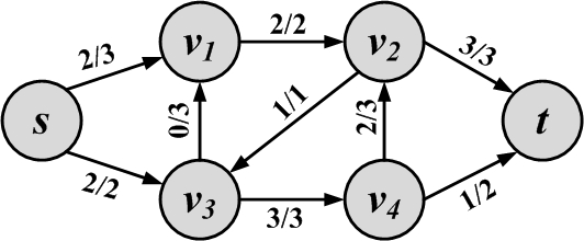
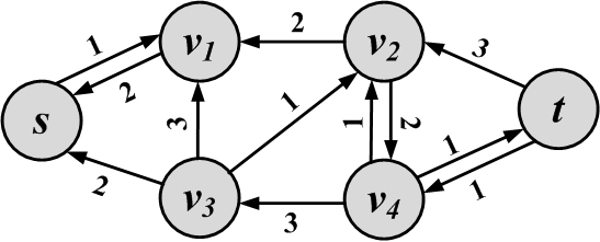
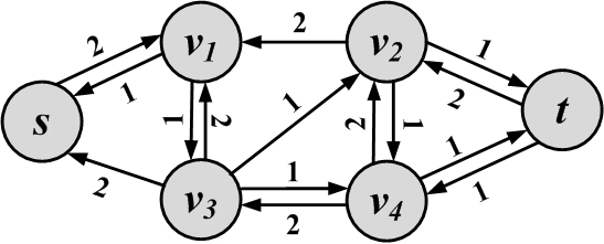
Consider the graph in Figure 2.24(b) and the augmenting path s, v_1, v_3, v_4, v_2, t. It has a minimum capacity of 1 along the path, so the flow quantity will be 1. We can augment the original graph with this path. The new flow graph and its corresponding residual graph are shown in Figure 2.25. In the new residual, no more augmenting paths can be found.
The Ford-Fulkerson algorithm will find the maximum flow in a network, but we skip the proof of optimality. Interested readers can refer to the bibliographic notes for proof of optimality and further information. The algorithm is provided in Algorithm 2.6.
- Require: Connected weighted graph G(V,E,W), Source s, Sink t
- return A Maximum flow graph
- $
- for all do (u,v) \in E, f(u,v)=0$
- while there exists an augmenting path p in the residual graph G_R do
- Augment flows by p
- end while
- Return flow value and flow graph;
The algorithm searches for augmenting paths, if possible, in the residual and augments flows in the original flow network. Path finding can be achieved by any graph traversal algorithm, such as BFS.
2.6.5 Maximum Bipartite Matching
Suppose we are trying to solve the following problem in social media:
Given n products and m users such that some users are only interested in certain products, find the maximum number of products that can be bought by users.
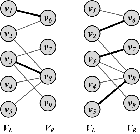
The problem is graphically depicted in Figure 2.26. The nodes on the left represent products and the nodes on the right represent users. Edges represent the interest of users in products. Highlighted edges demonstrate a matching
Matching, where products are matched with users. The figure on the left depicts a matching and the figure on the right depicts a maximum matching, where no more edges can be added to increase the size of the matching.
This problem can be reformulated as a bipartite graph problem. Given a bipartite graph, where V_L and V_R represent the left and right node sets (V = V_L \cup V_R), and E represents the edges, we define a matching M, M \subset E, such that, for all v \in V, d_v \le 1. In other words, either the node is matched (d_v = 1) or not (d_v=0). A maximum bipartite matching M_{Max} is a matching such that, for any other matching M' in the graph, |M_{Max}| \ge |M'|.
Here we solve the maximum bipartite matching problem using the previously discussed Ford-Fulkerson maximum flow technique. The problem can be easily solved by creating a flow graph G(V',E',C) from our bipartite graph G(V,E), as follows:
Set V' = V \cup \{s\} \cup \{t\}.
Connect all nodes in V_L to s and all nodes in V_R to t,
E'=E \cup \{(s,v)|v \in V_L\} \cup \{(v,t)| v \in V_R\}.(2.32)Set c(u,v) = 1, \forall (u,v) \in E^{\prime}.
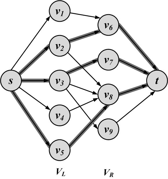
This procedure is graphically shown in Figure 2.27. By solving the max flow for this flow graph, the maximum matching is obtained, since the maximum number of edges need to be used between V_L and V_R for the flow to become maximum.4
2.6.6 Bridge Detection
As discussed in Section 1.5.7, bridges or cut edges
Cut-Edgesare edges whose removal makes formerly connected components disconnected. Here we list a simple algorithm for detecting bridges. This algorithm is computationally expensive, but quite intuitive. More efficient algorithms have been described for the same task.
Since we know that, by removing bridges, formerly connected components become disconnected, one simple algorithm is to remove edges one by one and test if the connected components become disconnected. This algorithm is outlined in Algorithm 2.7.
- Require: Connected graph G(V,E)
- return Bridge Edges
- bridgeSet = \{\}
- for e(u,v) \in E do
- G' = Remove e from G
- Disconnected = False;
- if BFS in G' starting at u does not visit v then
- Disconnected = True;
- end if
- if Disconnected then
- bridgeSet = bridgeSet \cup \{e\}
- end if
- end for
- Return bridgeSet
The disconnectedness of a component whose edge e(u,v) is removed can be analyzed by means of any graph traversal algorithm (e.g., BFS or DFS). Starting at node u, we traverse the graph using BFS and, if node v cannot be visited (Line 6), the component has been disconnected and edge e is a bridge (Line 10).
2.7 Summary
This chapter covered the fundamentals of graphs, starting with a presentation of the fundamental building blocks required for graphs: first nodes and edges, and then properties of graphs such as degree and degree distribution. Any graph must be represented using some data structure for computability. This chapter covered three well-established techniques: adjacency matrix, adjacency list, and edge list. Due to the sparsity of social networks, both adjacency list and edge list are more efficient and save significant space when compared to adjacency matrix. We then described various types of graphs: null and empty graphs, directed/undirected/mixed graphs, simple/multigraphs, and weighted graphs. Signed graphs are examples of weighted graphs that can be used to represent contradictory behavior.
We discussed connectivity in graphs and concepts such as paths, walks, trails, tours, and cycles. Components are connected subgraphs. We discussed strongly and weakly connected components. Given the connectivity of a graph, one is able to compute the shortest paths between different nodes. The longest shortest path in the graph is known as the diameter. Special graphs can be formed based on the way nodes are connected and the degree distributions. In complete graphs, all nodes are connected to all other nodes, and in regular graphs, all nodes have an equal degree. A tree is a graph with no cycle. We discussed two special trees: the spanning tree and the Steiner tree. Bipartite graphs can be partitioned into two sets of nodes, with edges between these sets and no edges inside these sets. Affiliation networks are examples of bipartite graphs. Bridges are single-point-of-failure edges that can make previously connected graphs disconnected.
In the section on graph algorithms, we covered a variety of useful techniques. Traversal algorithms provide an ordering of the nodes of a graph. These algorithms are particularly useful in checking whether a graph is connected or in generating paths. Shortest path algorithms find paths with the shortest length between a pair of nodes; Dijkstra’s algorithm is an example. Spanning tree algorithms provide subgraphs that span all the nodes and select edges that sum up to a minimum value; Prim’s algorithm is an example. The Ford-Fulkerson algorithm, is one of the maximum flow algorithms. It finds the maximum flow in a weighted capacity graph. Maximum bipartite matching is an application of maximum flow that solves a bipartite matching problem. Finally, we provided a simple solution for bridge detection.
2.8 Bibliographic Notes
The algorithms detailed in this chapter are from three well-known fields: graph theory, network science, and social network analysis. Interested readers can get better insight regarding the topics in this chapter by referring to general references in graph theory (Bondy and Murty 1976; West et al. 2001; Diestel 2005), algorithms and algorithm design (Kleinberg and Tardos, n.d.; Cormen 2001), network science (Newman 2010), and social network analysis (Wassermann and Faust 1994).
Other algorithms not discussed in this chapter include graph coloring (Jensen and Toft 1995), (quasi) clique detection (Abello et al. 2002), graph isomorphism (McKay 1981), topological sort algorithms (Cormen 2001), and the traveling salesman problem (TSP) (Cormen 2001), among others. In graph coloring, one aims to color elements of the graph such as nodes and edges such that certain constraints are satisfied. For instance, in node coloring the goal is to color nodes such that adjacent nodes have different colors. Cliques are complete subgraphs. Unfortunately, solving many problems related to cliques, such as finding a clique that has more that a given number of nodes, is NP-complete. In clique detection, the goal is to solve similar clique problems efficiently or provide approximate solutions. In graph isomorphism, given two graphs G and G', our goal is to find a mapping f from nodes of G to G' such that for any two nodes of G that are connected, their mapped nodes in G' are connected as well. In topological sort algorithms, a linear ordering of nodes is found in a directed graph such that for any directed edge (u,v) in the graph, node u comes before node v in the ordering. In the traveling salesman problem (TSP), we are provided cities and pairwise distances between them. In graph theory terms, we are given a weighted graph where nodes represent cities and edge weights represent distances between cities. The problem is to find the shortest walk that visits all cities and returns to the origin city.
Other noteworthy shortest path algorithms such as the A^* (Hart et al. 1968), the Bellman-Ford (BELLMA 1956), and all-pair shortest path algorithms such as Floyd-Warshall’s (Floyd 1962) are employed extensively in other literature.
In spanning tree computation, the Kruskal Algorithm (Kruskal 1956) or Boruvka (Motwani and Raghavan 2010) are also well-establishedalgorithms.
General references for flow algorithms, other algorithms not discussed in this chapter such as the Push-Relabel algorithm, and their optimality can be found in (Cormen 2001; Ahuja et al. 1995).
2.9 Exercises
~~~~~~~~~~Graph Basics
Given a directed graph G(V,E) and its adjacency matrix A, we propose two methods to make G undirected,
A'_{ij} = \min(1,A_{ij}+A_{ji}),(2.33)A'_{ij} = A_{ij} \times A_{ji},(2.34)where A'_{i,j} is the (i,j) entry of the undirected adjacency matrix. Discuss the advantages and disadvantages of each method.Graph Representation
Is it possible to have the following degrees in a graph with 7 nodes?
\{4,4,4,3,5,7,2\}.(2.35)Given the following adjacency matrix, compute the adjacency list and the edge list.
A= \left[ \begin{array}{ccccccccc} 0&1&1&0&0&0&0&0&0\\ 1&0&1&0&0&0&0&0&0\\ 1&1&0&1&1&0&0&0&0\\ 0&0&1&0&1&1&1&0&0\\ 0&0&1&1&0&1&1&0&0\\ 0&0&0&1&1&0&1&1&0\\ 0&0&0&1&1&1&0&1&0\\ 0&0&0&0&0&1&1&0&1\\ 0&0&0&0&0&0&0&1&0 \end{array}\right](2.36)2.9.1 Special Graphs
Prove that |E|= |V|-1 in trees.
2.9.2 Graph/Network Algorithms
Consider the tree shown in Figure 2.28. Traverse the graph using both BFS and DFS and list the order in which nodes are visited in each algorithm.
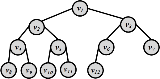
Figure 2.28: A Sample (Binary) Tree For a tree and a node v, under what condition is v visited sooner by BFS than DFS? Provide details.
For a real-world social network, is BFS or DFS more desirable? Provide details.
Compute the shortest path between any pair of nodes using Dijkstra’s algorithm for the graph in Figure 2.29.
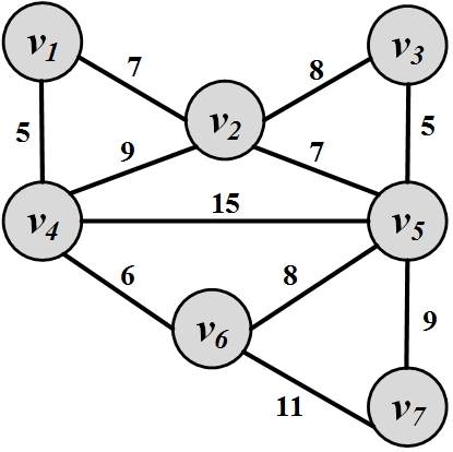
Figure 2.29: Weighted Graph. Detail why edges with negative weights are not desirable for computing shortest paths using Dijkstra’s algorithm.
Compute the minimal spanning tree using Prim’s algorithm in the graph provided in Figure 2.30.
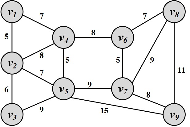
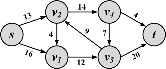
Figure 2.30: Weighted Graph Compute the maximum flow in Figure 2.31.
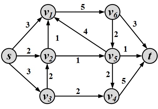
Figure 2.31: Flow Graph Given a flow network, you are allowed to change one edge’s capacity. Can this increase the flow? How can we find the correct edge to change?
How many bridges are in a bipartite graph? Provide details.
This is similar to plotting the probability mass function for degrees.↩︎
Instead of W in weighted networks, C is used to clearly represent capacities.↩︎
This edge is often called the weak link.↩︎
The proof is omitted here and is a direct result from the minimum-cut/maximum flow theorem not discussed in this chapter.↩︎